GATE EC · EE · IN

Compensators and PID controllers

Compensators (lead, lag and lead-lag) and PID controllers are blocks added in cascade with a plant when adjusting one gain cannot meet the steady-state and transient specifications together. These notes show how to tell lead from lag by the pole-zero pattern, find the maximum phase and the frequency where it occurs, predict what P, I and D action do to system type, steady-state error, damping and noise, size passive RC and op-amp networks, design lead and lag networks from the Bode plot, and apply the Ziegler-Nichols tuning tables. Each formula below only works in the form (convention) stated beside it.

10 previous-year questions · 10 solved · 6 practice questions

Why compensate: what each frequency band controls

A compensator $G_{c} (s)$ sits in cascade with the plant $G (s)$ in the forward path of a unity negative-feedback loop, so the loop transfer function becomes $G_{c} (s) G (s)$ . With a plain gain $K$ you face a trade-off. Raising $K$ reduces steady-state error, but for many plants it also lowers the phase margin and the damping. A compensator removes this trade-off because it shapes the loop differently at different frequencies.

Read the open-loop frequency response in three bands

Low band ( $ω \to 0$ ): sets the error constants and therefore the steady-state error. Integral and lag action work here.
Middle band (around the gain crossover frequency $ω_{g c}$ ): sets the phase margin, damping, overshoot and speed of response. Lead and derivative action work here.
High band: decides how much sensor noise reaches the actuator and the output. Derivative and lead action raise the gain here; lag and integral action lower it.

Conventions used in these notes: unity negative feedback, $e = r - y$ , phase counted positive for lead, and error constants always computed from the compensated loop $G_{c} (s) G (s)$ . The position error constant is written $K_{pos}$ so it cannot be confused with the proportional gain $K_{p}$ .

ERROR CONSTANTS AND STEADY-STATE ERROR

K_{pos} e_{ss, step} = s \to 0 lim G_{c} (s) G (s), K_{v} = s \to 0 lim s G_{c} (s) G (s), K_{a} = s \to 0 lim s^{2} G_{c} (s) G (s) = \frac{A}{1 + K _{pos}}, e_{ss, ramp} = \frac{A}{K _{v}}, e_{ss, parabola} = \frac{A}{K _{a}}

Applies to unity feedback with a stable closed loop, for inputs $A u (t)$ , $A t u (t)$ and $\frac{A}{2} t^{2} u (t)$ . A type- $N$ loop ( $N$ poles at the origin) has zero error for inputs of lower order than $t^{N}$ , a finite error for $t^{N}$ , and an infinite error for higher orders.

CONVERTING A DAMPING SPECIFICATION INTO A PHASE MARGIN

PM = tan^{- 1} \frac{2 ζ}{1 + 4 ζ ^{4} - 2 ζ ^{2}}, ω_{g c} = ω_{n} 1 + 4 ζ^{4} - 2 ζ^{2}, PM \approx 100 ζ degrees

Exact for the unity-feedback loop $\frac{ω _{n}^{2}}{s ( s + 2 ζ ω _{n} )}$ , whose closed loop is a pure second-order system. The straight-line rule $PM \approx 100 ζ$ degrees stays within about $3. 5^{\circ}$ of the exact value for $0 < ζ \leq 0.6$ and drifts off above that ( $ζ = 0.7$ gives $65. 2^{\circ}$ , not $7 0^{\circ}$ ). For a higher-order loop it is only an estimate, valid when one complex pole pair dominates. Lead and lag design from the Bode plot start by turning a $ζ$ or overshoot specification into a required PM this way.

P, I and D actions; PI, PD and PID controllers

PID CONTROL LAW (TIME DOMAIN)

u (t) = K_{p} e (t) + K_{i} \int_{0}^{t} e (τ) d τ + K_{d} \frac{d e ( t )}{d t}

Parallel (ideal) form. The P term responds to the present error, the I term to the error accumulated so far, and the D term to how fast the error is changing, which anticipates where it is heading. $K_{i} = K_{p} / T_{i}$ and $K_{d} = K_{p} T_{d}$ , where $T_{i}$ is the integral (reset) time and $T_{d}$ is the derivative time.

PID TRANSFER FUNCTION

G_{c} (s) = K_{p} + \frac{K _{i}}{s} + K_{d} s = K_{p} (1 + \frac{1}{T _{i} s} + T_{d} s) = \frac{K _{d} s ^{2} + K _{p} s + K _{i}}{s}

Has one pole at the origin and two zeros, the roots of $K_{d} s^{2} + K_{p} s + K_{i} = 0$ . The zeros are real when $K_{p}^{2} \geq 4 K_{i} K_{d}$ (equivalently $T_{i} \geq 4 T_{d}$ ) and a complex pair otherwise. With $K_{i} \neq = 0$ it raises the system type by 1.

PI CONTROLLER

G_{c} (s) = K_{p} + \frac{K _{i}}{s} = K_{p} (1 + \frac{1}{T _{i} s}) = \frac{K _{p} ( s + \frac{1}{T _{i}} )}{s}

Assumes $K_{p} > 0$ and $T_{i} > 0$ . Pole at $s = 0$ and zero at $s = - 1/ T_{i} = - K_{i} / K_{p}$ . Phase $= - tan^{- 1} \frac{1}{ω T _{i}}$ , which lies between $- 9 0^{\circ}$ and $0^{\circ}$ . Raises the type by 1.

PD CONTROLLER

G_{c} (s) = K_{p} + K_{d} s = K_{p} (1 + T_{d} s)

Assumes $K_{p} > 0$ and $T_{d} > 0$ . Zero at $s = - 1/ T_{d} = - K_{p} / K_{d}$ and no pole. Phase $= + tan^{- 1} (ω T_{d})$ , which lies between $0^{\circ}$ and $+ 9 0^{\circ}$ . The system type does not change.

PHASE OF A PID CONTROLLER

∠ G_{c} (j ω) = tan^{- 1} (\frac{K _{d} ω - K _{i} / ω}{K _{p}}), ∠ G_{c} = 0 at ω_{0} = \frac{K _{i}}{K _{d}} = \frac{1}{T _{i} T _{d}}

Assumes $K_{p}$ , $K_{i}$ and $K_{d}$ are all positive. Below $ω_{0}$ the integral term dominates and the controller lags; above $ω_{0}$ the derivative term dominates and it leads. The phase tends to $- 9 0^{\circ}$ as $ω \to 0$ and to $+ 9 0^{\circ}$ as $ω \to \infty$ .

What each action does

Action	Adds to the loop	Type and steady-state error	Damping and stability	Noise
P: $K_{p}$	Gain only, no pole or zero; $0^{\circ}$	Type unchanged. A finite error falls as $K_{p}$ rises (step into a type-0 plant of DC gain $K$ : $e_{ss} = \frac{A}{1 + K _{p} K}$ ) but never reaches zero	For many plants a higher $K_{p}$ lowers the damping and the phase margin; for a plant of order three or more, or one with dead time, a large enough $K_{p}$ can make the loop unstable	Passed on, scaled by $K_{p}$
I: $K_{i} / s$	Pole at $s = 0$ ; $- 9 0^{\circ}$	Type raised by 1, provided the closed loop stays stable: an error that was finite becomes zero (step error for type 0, ramp error for type 1)	Lowers the phase margin and makes the response more oscillatory; the order rises; can destabilise	Gain falls with frequency, so noise is attenuated
D: $K_{d} s$	Zero (at $s = 0$ alone, at $- 1/ T_{d}$ in PD); $+ 9 0^{\circ}$	Used in PD or PID: type unchanged and no direct effect, because D responds only to a changing error. Used alone, its zero at $s = 0$ cancels a plant integrator and worsens the error	Adds damping, reduces overshoot, improves relative stability	Gain rises with frequency, so noise is amplified

P CONTROL OF A TYPE-1 SECOND-ORDER PLANT

G_{c} (s) G (s) = \frac{K _{p} K}{s ( s + a )} : ω_{n} = K_{p} K, ζ = \frac{a}{2 K _{p} K}, K_{v} = \frac{K _{p} K}{a}

Unity feedback, $K_{p} K > 0$ , $a > 0$ . Shows the gain trade-off. A larger $K_{p}$ raises $K_{v}$ (smaller ramp error) and $ω_{n}$ , but lowers $ζ$ (more overshoot).

DERIVATIVE (PD) CONTROL OF A SECOND-ORDER PLANT

G (s) = \frac{ω _{n}^{2}}{s ( s + 2 ζ ω _{n} )}, G_{c} (s) = 1 + T_{d} s : ζ^{'} = ζ + \frac{ω _{n} T _{d}}{2}

The closed-loop characteristic equation becomes $s^{2} + (2 ζ ω_{n} + ω_{n}^{2} T_{d}) s + ω_{n}^{2} = 0$ . So $ω_{n}$ and $K_{v} = ω_{n} / (2 ζ)$ are unchanged and the damping increases. The closed loop also gains a zero at $s = - 1/ T_{d}$ . For an underdamped $ζ^{'}$ this zero makes the response rise faster and overshoot more than a pure second-order system with the same $ζ^{'}$ , and the effect is stronger the closer the zero lies to the origin compared with $ζ^{'} ω_{n}$ .

RATE (TACHOMETER) FEEDBACK, FOR COMPARISON

G (s) = \frac{ω _{n}^{2}}{s ( s + 2 ζ ω _{n} )} with minor loop K_{t} s : ζ^{'} = ζ + \frac{K _{t} ω _{n}}{2}, K_{v} = \frac{ω _{n}}{2 ζ + K _{t} ω _{n}}

The inner loop reduces to $\frac{ω _{n}^{2}}{s ( s + 2 ζ ω _{n} + K _{t} ω _{n}^{2} )}$ , so the characteristic equation is the same as with PD and $T_{d} = K_{t}$ , and there is no closed-loop zero. But $K_{v}$ falls below $ω_{n} / (2 ζ)$ , so the ramp error grows. PD in the forward path keeps $K_{v}$ unchanged.

PD is the limiting case of a lead compensator (its pole pushed out to $- \infty$ ). PI is the limiting case of a lag compensator (its pole pushed in to the origin). That is why lead and PD are used for the transient response, and lag and PI for steady-state accuracy. PID combines the two, in the same way a lead-lag compensator does.

OP-AMP PI AND PD CONTROLLERS (INVERTING STAGE)

PI: Z_{1} = R_{1}, Z_{2} = R_{2} + \frac{1}{C _{2} s} : PD: Z_{1} = R_{1} ∥ C_{1}, Z_{2} = R_{2} : \frac{V _{o}}{V _{i}} = - \frac{R _{2}}{R _{1}} (1 + \frac{1}{R _{2} C _{2} s}) \frac{V _{o}}{V _{i}} = - \frac{R _{2}}{R _{1}} (1 + R_{1} C_{1} s)

Ideal op-amp, $\frac{V _{o}}{V _{i}} = - \frac{Z _{2}}{Z _{1}}$ with $Z_{1}$ the input impedance and $Z_{2}$ the feedback impedance. PI: $K_{p} = R_{2} / R_{1}$ and $T_{i} = R_{2} C_{2}$ . PD: $K_{p} = R_{2} / R_{1}$ and $T_{d} = R_{1} C_{1}$ . A second inverting stage of gain $- R_{4} / R_{3}$ removes the minus sign.

INTEGRAL ACTION CAN DESTABILISE

Take $G (s) = \frac{1}{s ( s + 1 )}$ with pure integral control $K_{i} / s$ . The characteristic equation is $s^{3} + s^{2} + K_{i} = 0$ . Its $s^{1}$ coefficient is missing, so the loop is unstable for every $K_{i} > 0$ . With PI control the equation is $s^{3} + s^{2} + K_{p} s + K_{i} = 0$ , and Routh shows it is stable only if $K_{p} > K_{i} > 0$ . In other words, the PI zero $- K_{i} / K_{p}$ must lie between the origin and the plant pole at $- 1$ .

EXAM TIP

Adding I raises the type by one, whatever the input, provided the compensated closed loop is stable. A type-0 plant with PI has zero step error and a finite ramp error $A / K_{v}$ , where $K_{v} = K_{i} G (0)$ . A type-1 plant with PI has zero ramp error and a finite parabolic error.

EXAM TIP

Derivative action is never used on its own. A constant error gives zero derivative output, so D alone cannot hold the output at a set point, and its zero at the origin cancels a plant integrator. The ideal term $K_{d} s$ is also improper, so practical controllers use a filtered derivative $\frac{K _{d} s}{1 + ( T _{d} / N ) s}$ , which limits the derivative term's high-frequency gain to $K_{p} N$ .

Process-control terms

Proportional band: $PB = \frac{100}{K _{p}} %$ , where $K_{p}$ is the dimensionless gain with the error and the controller output both expressed as percentages of their full ranges. PB is the error span that drives the output across its full range, so a narrow band means a high gain.
Offset: P-only control of a type-0 process leaves a steady-state error after a set-point or load change (the P row of the table above). Integral action removes it.
Integral (reset) time $T_{i}$ : for a constant error $e$ , the I term grows by $K_{p} e / T_{i}$ per unit time, so after a time $T_{i}$ it has repeated the P output once. Its reciprocal $1/ T_{i}$ is the reset rate, in repeats per unit time.
Derivative (rate) time $T_{d}$ : for a ramp error $e = r t$ , PD gives $K_{p} r (t + T_{d})$ , which is what P alone would give $T_{d}$ later. PD anticipates the error by $T_{d}$ .
Integral windup: while the actuator is saturated, the integral term keeps accumulating error, so the output overshoots and recovers slowly after the error changes sign. Anti-windup schemes stop or limit integration during saturation.

Lead compensator

Convention used here: $G_{c} (s) = \frac{1 + a T s}{1 + T s}$ with $a > 1$ . This form has unity DC gain and high-frequency gain $a$ . The same network is also written $\frac{1 + T s}{1 + α T s}$ with $0 < α < 1$ , or in pole-zero form $\frac{s + z}{s + p}$ with $0 < z < p$ . Results for all three forms are given below; first work out which form a question uses.

The zero at $- 1/ (a T)$ is nearer the origin than the pole at $- 1/ T$ . On the Bode plot the zero corner comes first, so the phase rises, and then the pole corner pulls it back down. The phase is positive at every frequency and peaks midway between the two corners on a log scale.

LEAD COMPENSATOR (TIME-CONSTANT FORM)

G_{c} (s) = \frac{1 + a T s}{1 + T s}, a > 1; zero at - \frac{1}{a T}, pole at - \frac{1}{T}

Corner frequencies are $\frac{1}{a T}$ (zero) and $\frac{1}{T}$ (pole). The gain rises from 1 (0 dB) at low frequency to $a$ ( $20 lo g_{10} a$ dB) at high frequency, which is a high-pass shape.

PHASE OF THE LEAD COMPENSATOR AT ANY FREQUENCY

ϕ (ω) = tan^{- 1} (aω T) - tan^{- 1} (ω T) = tan^{- 1} \frac{( a - 1 ) ω T}{1 + a ω ^{2} T ^{2}}

Positive for all $ω > 0$ when $a > 1$ .

MAXIMUM PHASE LEAD

sin ϕ_{m} = \frac{a - 1}{a + 1}, tan ϕ_{m} = \frac{a - 1}{2 a}, a = \frac{1 + sin ϕ _{m}}{1 - sin ϕ _{m}}

Valid for the time-constant form with $a > 1$ . $ϕ_{m}$ depends only on the ratio $a$ of the two corner frequencies, not on $T$ . For any finite $a$ , $ϕ_{m} < 9 0^{\circ}$ .

FREQUENCY OF MAXIMUM PHASE LEAD

ω_{m} = \frac{1}{T a} = \frac{1}{a T} \cdot \frac{1}{T}

The geometric mean of the two corner frequencies, which is their midpoint on a log scale.

GAIN AT THE FREQUENCY OF MAXIMUM LEAD

∣ G_{c} (j ω_{m}) ∣ = a i.e. 10 lo g_{10} a dB

Holds for the unity-DC-gain form. In lead design, $ω_{m}$ is placed at the new gain crossover, where the uncompensated magnitude is $- 10 lo g_{10} a$ dB.

OTHER FORMS OF THE LEAD COMPENSATOR

\frac{1 + T s}{1 + α T s}, 0 < α < 1 : \frac{s + z}{s + p}, 0 < z < p : sin ϕ_{m} = \frac{1 - α}{1 + α}, ω_{m} = \frac{1}{T α} sin ϕ_{m} = \frac{p - z}{p + z}, ω_{m} = z p, ∣ G_{c} (j ω_{m}) ∣ = \frac{z}{p}

$α = 1/ a$ . The pole-zero form has DC gain $z / p < 1$ and high-frequency gain 1. Its phase is identical to the time-constant form with the same corners.

WHERE THE MAXIMUM-LEAD FORMULA COMES FROM

As $ω$ goes from 0 to $\infty$ , $G_{c} (j ω) = \frac{1 + j aω T}{1 + j ω T}$ traces a semicircle in the upper half-plane from 1 to $a$ , with centre $\frac{a + 1}{2}$ and radius $\frac{a - 1}{2}$ . The largest angle is where a line from the origin just touches the circle, so $sin ϕ_{m} = \frac{radius}{centre} = \frac{a - 1}{a + 1}$ . The distance from the origin to that point is $centre^{2} - radius^{2} = a$ , which is $∣ G_{c} (j ω_{m}) ∣$ .

Effects of lead compensation. It adds positive phase near the gain crossover, so the phase margin rises and the response is better damped, with less overshoot. Its high-frequency gain pushes the gain crossover frequency up, so the bandwidth increases and the response gets faster, with shorter rise and settling times. On the root locus the zero-pole pair adds a net positive angle and bends the locus to the left, which improves relative stability. In the unity-DC-gain form it leaves the error constants unchanged, so it does not directly reduce steady-state error. In the pole-zero form $\frac{s + z}{s + p}$ its DC gain is $z / p < 1$ , so the loop gain must be raised by $p / z$ just to keep the same error constant. Any gain in accuracy is indirect: the extra phase margin lets you use a larger $K$ . The cost is more amplification of high-frequency noise and larger actuator signals.

PASSIVE RC LEAD NETWORK

\frac{V _{o} ( s )}{V _{i} ( s )} = \frac{R _{2} ( 1 + R _{1} C s )}{R _{1} + R _{2} + R _{1} R _{2} C s} = \frac{s + \frac{1}{R _{1} C}}{s + \frac{1}{R _{1} C} + \frac{1}{R _{2} C}} = \frac{1}{a} \cdot \frac{1 + a T s}{1 + T s}

Series arm: $R_{1}$ in parallel with $C$ . Shunt arm: $R_{2}$ across the output. Assumes an ideal source and an unloaded output. $a = \frac{R _{1} + R _{2}}{R _{2}}$ , $a T = R_{1} C$ , $T = \frac{R _{1} R _{2} C}{R _{1} + R _{2}}$ . The network attenuates DC by $1/ a$ , so an amplifier of gain $a$ is needed to keep the error constant.

Lead design from the Bode plot

Convert the transient specification into a required phase margin (for example $PM \approx 100 ζ$ degrees).
Set the loop gain $K$ to meet the error-constant specification.
Draw the Bode plot of $K G (j ω)$ and read the uncompensated phase margin.
Required lead: $ϕ_{m} = PM_{required} - PM_{uncompensated} + (5^{\circ} to 1 2^{\circ})$ . The extra allows for the phase the plant loses when the crossover moves to a higher frequency.
Compute $a = \frac{1 + sin ϕ _{m}}{1 - sin ϕ _{m}}$ .
The new gain crossover $ω_{g c}^{'}$ is the frequency where $∣ K G (j ω) ∣ = - 10 lo g_{10} a$ dB. Set $ω_{m} = ω_{g c}^{'}$ .
$T = \frac{1}{ω _{m} a}$ , which puts the zero corner at $\frac{1}{a T}$ and the pole corner at $\frac{1}{T}$ .
Check the compensated phase margin. If it falls short, increase $ϕ_{m}$ and repeat.

Lead design on the root locus

From the specifications ( $0 < ζ < 1$ , $ω_{n}$ ), fix the desired dominant closed-loop pole $s_{d} = - ζ ω_{n} + j ω_{n} 1 - ζ^{2}$ .
Evaluate $∠ G (s_{d})$ . The compensator must supply $ϕ = - 18 0^{\circ} - ∠ G (s_{d})$ (modulo $36 0^{\circ}$ ). A positive $ϕ$ calls for a lead.
Place the zero and the pole on the negative real axis so that $∠ (s_{d} + z) - ∠ (s_{d} + p) = ϕ$ . If $ϕ$ is large, split it across two lead sections.
Find the gain from the magnitude condition $∣ K G_{c} (s_{d}) G (s_{d}) ∣ = 1$ , then check the error constant.

WHEN LEAD COMPENSATION STRUGGLES

Lead works poorly when the uncompensated phase falls steeply near the gain crossover. Moving the crossover up then costs almost as much phase as the network adds, so the phase margin barely improves and raising $a$ gains little. Lag or lead-lag compensation is used instead.

VALUES WORTH MEMORISING

$a = 3$ gives $ϕ_{m} = 3 0^{\circ}$ ; $a = 4$ gives $36.8 7^{\circ}$ ; $a = 3 + 22 \approx 5.83$ gives $4 5^{\circ}$ ; $a = 9$ gives $53.1 3^{\circ}$ ; $a \approx 13.93$ gives $6 0^{\circ}$ . The required $a$ grows steeply as $ϕ_{m}$ approaches $9 0^{\circ}$ , which is why a large phase requirement is split across two lead sections in cascade.

LEAD OR LAG AT A GLANCE

In the pole-zero form $\frac{s + z}{s + p}$ with $z, p > 0$ : if the zero is nearer the origin ( $z < p$ ) it is a lead; if the pole is nearer the origin ( $p < z$ ) it is a lag. In the time-constant form $\frac{1 + τ _{1} s}{1 + τ _{2} s}$ : $τ_{1} > τ_{2}$ is a lead and $τ_{1} < τ_{2}$ is a lag. A positive constant multiplier does not change this.

Lag and lead-lag compensators

Convention used here: $G_{c} (s) = \frac{1 + T s}{1 + b T s}$ with $b > 1$ . Now the pole at $- 1/ (b T)$ is nearer the origin than the zero at $- 1/ T$ . The phase is negative at every frequency, and the gain falls from 1 at low frequency to $1/ b$ at high frequency, which is a low-pass shape. What makes a lag network useful is its attenuation, not its phase. Its corners are placed well below the gain crossover, so near crossover it simply lowers the gain by $20 lo g_{10} b$ dB and adds only a few degrees of lag.

LAG COMPENSATOR (TIME-CONSTANT FORM)

G_{c} (s) = \frac{1 + T s}{1 + b T s}, b > 1; zero at - \frac{1}{T}, pole at - \frac{1}{b T}

High-frequency gain is $1/ b$ , an attenuation of $20 lo g_{10} b$ dB above the zero corner.

MAXIMUM PHASE LAG

sin ϕ_{m} = - \frac{b - 1}{b + 1} at ω_{m} = \frac{1}{T b}

Same algebra as the lead, with the sign reversed. $ω_{m}$ is the geometric mean of the corners $\frac{1}{b T}$ and $\frac{1}{T}$ .

LAG IN POLE-ZERO FORM AND ITS EFFECT ON STEADY-STATE ERROR

G_{c} (s) = \frac{s + z}{s + p}, z > p > 0 : K_{v}^{new} = \frac{z}{p} K_{v}^{old} (likewise K_{pos}, K_{a})

Holds at the same loop gain $K$ , for a stable compensated loop. DC gain is $z / p$ and high-frequency gain is 1. When $z$ and $p$ both sit close to the origin (a dipole), the angle they add at the dominant poles is small. The transient response then barely changes while the error constant is multiplied by $z / p$ .

PASSIVE RC LAG NETWORK

\frac{V _{o} ( s )}{V _{i} ( s )} = \frac{1 + R _{2} C s}{1 + ( R _{1} + R _{2} ) C s}, T = R_{2} C, b = \frac{R _{1} + R _{2}}{R _{2}}

Series arm: $R_{1}$ . Shunt arm: $R_{2}$ in series with $C$ , with the output taken across this shunt arm. Assumes an unloaded output. DC gain is 1, so no amplifier is needed to hold the low-frequency gain.

OP-AMP LEAD OR LAG NETWORK

\frac{V _{o}}{V _{i}} = \frac{R _{2} R _{4}}{R _{1} R _{3}} \cdot \frac{1 + R _{1} C _{1} s}{1 + R _{2} C _{2} s} (Z_{1} = R_{1} ∥ C_{1}, Z_{2} = R_{2} ∥ C_{2}, then an inverter of gain - R_{4} / R_{3})

Ideal op-amps. The first inverting stage gives $- \frac{R _{2}}{R _{1}} \cdot \frac{1 + R _{1} C _{1} s}{1 + R _{2} C _{2} s}$ and the second stage cancels the sign. Zero at $- 1/ (R_{1} C_{1})$ , pole at $- 1/ (R_{2} C_{2})$ : a lead if $R_{1} C_{1} > R_{2} C_{2}$ and a lag if $R_{1} C_{1} < R_{2} C_{2}$ . Unlike the passive networks, the DC gain $\frac{R _{2} R _{4}}{R _{1} R _{3}}$ can be set independently of the pole-zero ratio.

Effects of lag compensation. The network leaves the low-frequency gain alone and cuts the gain near crossover by $b$ . So the loop gain $K$ can be set as high as the error-constant specification demands, and the network then pulls the gain crossover down to a frequency where the plant's phase is less negative, which restores the phase margin. Compared with the uncompensated system at the same $K$ , the crossover and bandwidth are lower, so the response is slower. The slow pole-zero dipole also leaves a small, slowly decaying tail in the step response. High-frequency noise is attenuated.

Lag design from the Bode plot

Set $K$ to meet the error-constant specification.
Find the frequency $ω_{g c}^{'}$ where the phase of $K G (j ω)$ equals $- 18 0^{\circ} + PM_{required} + (5^{\circ} to 1 2^{\circ})$ . The extra covers the lag the network still adds at that frequency.
Choose $b$ so the network cancels the magnitude there: $20 lo g_{10} b = ∣ K G (j ω_{g c}^{'}) ∣$ in dB.
Put the zero corner about a decade below the new crossover, $\frac{1}{T} \approx \frac{ω _{g c}^{'}}{10}$ . The pole corner is then at $\frac{1}{b T}$ .
Check the phase margin and the error constant.

Lead-lag compensation places a lag section in cascade with a lead section. The lag section works at low frequencies, for steady-state accuracy; the lead section works near crossover, for phase margin and speed. Use it when both the error specification and the transient specification are beyond what one section can deliver.

LEAD-LAG COMPENSATOR

G_{c} (s) = \frac{1 + T _{2} s}{1 + b T _{2} s} \cdot \frac{1 + a T _{1} s}{1 + T _{1} s}, a > 1, b > 1, \frac{1}{T _{2}} ≪ \frac{1}{a T _{1}}

The first factor is the lag section and the second is the lead section. Both lag corners lie well below both lead corners.

PASSIVE LAG-LEAD NETWORK (SINGLE RATIO)

G_{c} (s) = \frac{( 1 + T _{1} s ) ( 1 + T _{2} s )}{( 1 + \frac{T _{1}}{β} s ) ( 1 + β T _{2} s )}, β > 1, T_{2} > T_{1}; ∠ G_{c} = 0 at ω_{0} = \frac{1}{T _{1} T _{2}}

Realised by one RC network: series arm $R_{1}$ in parallel with $C_{1}$ , shunt arm $R_{2}$ in series with $C_{2}$ , output across the shunt arm, unloaded. Then $T_{1} = R_{1} C_{1}$ and $T_{2} = R_{2} C_{2}$ , and the denominator $1 + (R_{1} C_{1} + R_{2} C_{2} + R_{1} C_{2}) s + R_{1} C_{1} R_{2} C_{2} s^{2}$ factors as $(1 + \frac{T _{1}}{β} s) (1 + β T_{2} s)$ , so the lead and lag sections are forced to share the same ratio $β$ . The phase is a lag below $ω_{0}$ and a lead above it. DC and high-frequency gains are both 1, with a dip in between.

Lead vs lag vs lead-lag

Property	Lead	Lag	Lead-lag
Pole-zero form $\frac{s + z}{s + p}$	$z < p$ : zero nearer the origin	$p < z$ : pole nearer the origin	One pair of each; the lag pair sits at lower frequency
Phase	Positive; peak $sin^{- 1} \frac{a - 1}{a + 1}$	Negative; used for its attenuation, not its phase	Lag at low frequency, lead at high frequency
Magnitude shape	High-pass (gain rises by $a$ )	Low-pass (gain falls by $b$ )	Falls by $b$ across the lag corners, rises by $a$ across the lead corners (a mid-band dip back to 1 when $a = b$ )
Gain crossover and bandwidth	Increase	Decrease	Set by the design
Speed of response	Faster (rise and settling times fall)	Slower	Faster than lag alone
Phase margin and overshoot	PM rises because phase is added; overshoot falls	PM rises because crossover moves lower	PM rises
Steady-state error	No direct improvement	Error constants raised by up to $b$ (by $z / p$ in the pole-zero form at the same $K$ )	Improved by the lag section
Root locus	Bends the locus left, more stable	Locus near the dominant poles almost unchanged	Both effects
High-frequency noise	Amplified	Attenuated	Depends on the design
Controller analogue	PD	PI	PID

EXAM TIP

In the time-constant form, the lag network has unity DC gain and attenuates high frequencies, so $K$ is set by the error specification and the network's attenuation $1/ b$ brings the gain back down at the new crossover. In the pole-zero form $\frac{s + z}{s + p}$ , the network itself has DC gain $z / p$ . Both describe the same idea: more gain at low frequency than at crossover. Keep the lag corners well below crossover, otherwise the network's own phase lag eats into the phase margin it was meant to improve.

On-off control and Ziegler-Nichols tuning

On-off (two-position) control switches the actuator between two fixed levels: $u = U_{m a x}$ when $e > 0$ and $u = U_{m i n}$ when $e < 0$ . It is a nonlinear controller (an ideal relay). It is cheap and robust, and suits thermostats, level switches and similar processes where a small oscillation of the controlled variable is acceptable.

Properties of on-off control

The controlled variable never settles. It oscillates continuously about the set point (a limit cycle).
A differential gap (hysteresis) of width $h$ makes the controller switch at $e = + h /2$ and $e = - h /2$ instead of at $e = 0$ , which stops the actuator from chattering.
A wider differential gap gives a larger oscillation and a lower switching frequency: less actuator wear but poorer regulation. A narrower gap does the reverse.
Process lag and dead time make the output overshoot the switching points, so the oscillation is larger than the gap alone would give.

Ziegler-Nichols tuning gives starting values of $K_{p}$ , $T_{i}$ and $T_{d}$ for $G_{c} (s) = K_{p} (1 + \frac{1}{T _{i} s} + T_{d} s)$ from a simple experiment, without needing a model of the plant. The rules aim at a quarter-decay-ratio response, where each overshoot peak is about a quarter of the one before. Expect noticeable overshoot, and treat the settings as a starting point for fine tuning.

Method 1: step-response (process reaction curve) method

With the controller disconnected, apply a step to the plant in open loop. The method applies to plants whose step response is S-shaped (no integrator and no dominant complex poles).
Draw the tangent at the inflection point of the response. Where it cuts the time axis gives the apparent dead time $L$ . Where it meets the final-value line is $t = L + T$ , which gives the time constant $T$ .
This approximates the plant as $\frac{K e ^{- L s}}{T s + 1}$ , where $K$ is the steady-state output per unit step of input.
Read the settings from the table below.

Ziegler-Nichols settings, step-response method

Controller	$K_{p}$	$T_{i}$	$T_{d}$
P	$\frac{T}{K L}$	$\infty$	0
PI	$0.9 \frac{T}{K L}$	$\frac{L}{0.3} \approx 3.33 L$	0
PID	$1.2 \frac{T}{K L}$	$2 L$	$0.5 L$

EXAM TIP

$K$ is the process gain (steady-state change in output per unit change in input). For a reaction curve normalised to a final value of 1 ( $K = 1$ ), the gains reduce to the commonly printed $T / L$ , $0.9 T / L$ and $1.2 T / L$ . If a question gives the slope $R$ of the tangent (per unit step of input) instead of $T$ , use $R = K / T$ : the gains become $\frac{1}{R L}$ , $\frac{0.9}{R L}$ and $\frac{1.2}{R L}$ .

Method 2: ultimate-gain (sustained-oscillation) method

Close the loop with proportional control only ( $T_{i} = \infty$ , $T_{d} = 0$ ).
Raise $K_{p}$ from zero until the output just oscillates with constant amplitude. That gain is the ultimate (critical) gain $K_{u}$ , and the period of the oscillation is the ultimate period $P_{u}$ .
On paper, $K_{u}$ is the gain that puts closed-loop poles on the $j ω$ axis. In the Routh array, make the $s^{1}$ row zero; the auxiliary equation then gives $ω_{u}$ . Equivalently, $K_{u} = 1/∣ G (j ω_{p c}) ∣$ at the phase crossover frequency $ω_{p c}$ . Then $P_{u} = 2 π / ω_{u}$ .
The plant must be one that gain alone can drive into sustained oscillation, so its phase must reach $- 18 0^{\circ}$ at a finite frequency. The method cannot be used on, for example, a minimum-phase first- or second-order plant without dead time, because its phase never reaches $- 18 0^{\circ}$ .

Ziegler-Nichols settings, ultimate-gain method

Controller	$K_{p}$	$T_{i}$	$T_{d}$
P	$0.5 K_{u}$	$\infty$	0
PI	$0.45 K_{u}$	$\frac{P _{u}}{1.2} \approx 0.833 P_{u}$	0
PID	$0.6 K_{u}$	$0.5 P_{u}$	$0.125 P_{u}$

ZIEGLER-NICHOLS PID IN POLE-ZERO FORM

Step-response method (K = 1) : Ultimate-gain method: G_{c} (s) = 0.6 T \frac{( s + \frac{1}{L} ) ^{2}}{s} G_{c} (s) = 0.075 K_{u} P_{u} \frac{( s + \frac{4}{P _{u}} ) ^{2}}{s}

Both PID rows set $T_{i} = 4 T_{d}$ , which is exactly the condition $K_{p}^{2} = 4 K_{i} K_{d}$ for a double zero. So both give a pole at the origin and a double zero on the negative real axis, at $- 1/ L$ and at $- 4/ P_{u}$ respectively. The leading coefficient is $K_{d}$ , which makes a quick check. For a process gain $K \neq = 1$ , divide the step-response result by $K$ .

Worked examples

WORKED EXAMPLE · LEAD NETWORK: PHASE, GAIN AND RC VALUES

A lead compensator $G_{c} (s) = \frac{s + 2}{s + 8}$ is to be built as the passive RC lead network (series arm: $R_{1}$ in parallel with $C$ ; shunt arm: $R_{2}$ across the output) with $C = 10 μ F$ . Find (a) the maximum phase lead and the frequency at which it occurs, (b) the gain of $G_{c}$ at that frequency in dB, (c) $R_{1}$ and $R_{2}$ , and (d) the amplifier gain needed so that the loop's DC gain is not reduced.

Solution

This is the pole-zero form with $z = 2$ and $p = 8$ . The zero is nearer the origin, so it is a lead. In time-constant form, $\frac{s + 2}{s + 8} = \frac{1}{4} \cdot \frac{1 + 0.5 s}{1 + 0.125 s}$ , so $a = 4$ and $T = 0.125$ s.
(a) $sin ϕ_{m} = \frac{a - 1}{a + 1} = \frac{3}{5} = 0.6$ , so $ϕ_{m} = 36.8 7^{\circ}$ . It occurs at $ω_{m} = z p = 16 = 4$ rad/s. Check: $1/ (T a) = 1/ (0.125 \times 2) = 4$ .
(b) $∣ G_{c} (j 4) ∣ = \frac{4 ^{2} + 2 ^{2}}{4 ^{2} + 8 ^{2}} = \frac{20}{80} = 0.5$ , which is $20 lo g_{10} 0.5 = - 6.02$ dB. It splits into the $\frac{1}{4}$ factor ( $- 12.04$ dB) plus the $+ 10 lo g_{10} 4 = + 6.02$ dB of the unity-DC-gain lead.
(c) Zero: $\frac{1}{R _{1} C} = 2$ , so $R_{1} = \frac{1}{2 \times 1 0 ^{- 5}} = 50 k Ω$ . Pole: $\frac{1}{R _{1} C} + \frac{1}{R _{2} C} = 8$ , so $\frac{1}{R _{2} C} = 6$ and $R_{2} = \frac{1}{6 \times 1 0 ^{- 5}} \approx 16.67 k Ω$ . Check: $a = \frac{R _{1} + R _{2}}{R _{2}} = \frac{66.67}{16.67} = 4$ .
(d) The network's DC gain is $\frac{R _{2}}{R _{1} + R _{2}} = \frac{z}{p} = 0.25$ , so an amplifier of gain $a = 4$ restores it.

Answer: (a) $36.8 7^{\circ}$ at $4$ rad/s; (b) $- 6.02$ dB; (c) $R_{1} = 50 k Ω$ , $R_{2} \approx 16.67 k Ω$ ; (d) amplifier gain 4.

WORKED EXAMPLE · ZIEGLER-NICHOLS ULTIMATE-GAIN TUNING

The plant $G (s) = \frac{1}{s ( s + 2 ) ( s + 4 )}$ is under unity-feedback proportional control. Find the ultimate gain and period, then the Ziegler-Nichols PID settings. Write the controller as $K_{p} + K_{i} / s + K_{d} s$ and in pole-zero form.

Solution

Characteristic equation: $s (s + 2) (s + 4) + K = s^{3} + 6 s^{2} + 8 s + K = 0$ .
Routh array: $s^{3}$ : $1, 8$ ; $s^{2}$ : $6, K$ ; $s^{1}$ : $\frac{48 - K}{6}$ ; $s^{0}$ : $K$ . The $s^{1}$ row vanishes at $K_{u} = 48$ .
Auxiliary equation: $6 s^{2} + 48 = 0$ , so $s = \pm j 22$ and $ω_{u} = 22 = 2.828$ rad/s. Then $P_{u} = \frac{2 π}{ω _{u}} = \frac{π}{2} = 2.221$ s.
Cross-check with the frequency response. Setting the phase $- 9 0^{\circ} - tan^{- 1} \frac{ω}{2} - tan^{- 1} \frac{ω}{4} = - 18 0^{\circ}$ gives $\frac{ω ^{2}}{8} = 1$ , the same $ω = 22$ . There $∣ G (j 22) ∣ = \frac{1}{2 2 \cdot 12 \cdot 24} = \frac{1}{48}$ , so $K_{u} = 48$ .
From the table: $K_{p} = 0.6 K_{u} = 28.8$ , $T_{i} = 0.5 P_{u} = 1.111$ s, $T_{d} = 0.125 P_{u} = 0.2777$ s.
$K_{i} = \frac{K _{p}}{T _{i}} = \frac{28.8}{1.1107} = 25.93$ and $K_{d} = K_{p} T_{d} = 28.8 \times 0.27768 = 7.997 \approx 8.00$ .
Pole-zero form: $0.075 K_{u} P_{u} = 0.075 \times 48 \times 2.2214 = 8.00$ and $4/ P_{u} = 1.80$ , so $G_{c} (s) = \frac{8.00 ( s + 1.80 ) ^{2}}{s}$ . Expanding gives $\frac{8.00 s ^{2} + 28.8 s + 25.9}{s}$ , which matches.

Answer: $K_{u} = 48$ , $P_{u} = 2.221$ s; $K_{p} = 28.8$ , $T_{i} = 1.111$ s, $T_{d} = 0.278$ s; $G_{c} (s) \approx 28.8 + \frac{25.93}{s} + 8.00 s = \frac{8.00 ( s + 1.80 ) ^{2}}{s}$ .

Exam traps and shortcuts

IDENTIFY THE FORM FIRST

$sin ϕ_{m} = \frac{a - 1}{a + 1}$ is for $\frac{1 + a T s}{1 + T s}$ with $a > 1$ . For $\frac{1 + T s}{1 + α T s}$ with $α < 1$ it becomes $\frac{1 - α}{1 + α}$ , and for $\frac{s + z}{s + p}$ it is $\frac{p - z}{p + z}$ . Use the formula for the wrong form and you get a wrong angle or a wrong sign.

GEOMETRIC MEAN, NOT AVERAGE

The maximum phase of a lead or lag always occurs at the geometric mean of the two corner frequencies, $z p$ , never at their arithmetic mean. Scaling $z$ and $p$ by the same factor moves $ω_{m}$ but leaves $ϕ_{m}$ unchanged.

WHICH ONE DOES WHAT

Lead improves the transient: phase margin, speed and bandwidth all go up. Lag improves the steady state: error constants go up and bandwidth goes down. If a question says the compensator reduces bandwidth or filters noise, it is a lag. If it says the compensator speeds up the response, it is a lead.

REMOVING AN ERROR VS REDUCING IT

Only integral action (I, PI, PID) changes the system type, so only it can turn a finite steady-state error into zero. A lag network with its pole off the origin multiplies the error constant by a finite factor, which reduces the error but does not remove it. PD and lead action leave the type unchanged.

STABILITY BEFORE ERROR

Compute error constants with the compensator in the loop, and quote $e_{ss}$ only after confirming that the compensated closed loop is stable. An unstable loop has no steady state.

READING THE REACTION CURVE

In a Ziegler-Nichols step-response question, measure $T$ from where the tangent cuts the time axis ( $t = L$ ) to where it meets the final-value line ( $t = L + T$ ), not from $t = 0$ .

PREVIOUS-YEAR QUESTIONS

10 questions from the EC, EE and IN papers

Try each question first, then open the answer. We placed each question under a topic ourselves; the exam paper does not label topics.

See these papers in full: GATE ECE 2026 · GATE ECE 2025 · GATE ECE 2024 · GATE EE 2025 · GATE EE 2023 · GATE IN 2025 · GATE IN 2023 · GATE IN 2020

GATE 2026 EC Q.40

GATE 2026 · ECQ.40 · 2 marks · MCQ

For the control system shown in the Figure, the transfer function of a plant, $G (s) = \frac{1}{( s + 1 ) ( s + 2 )}$ is connected in cascade with a compensator $C (s) = K (s + α)$ , where $K$ and $α$ are positive real valued constants.

Which of the following pairs $(K, α)$ represent the correct values for the closed loop system to have poles at $(- 3 \pm j 5)$ ?

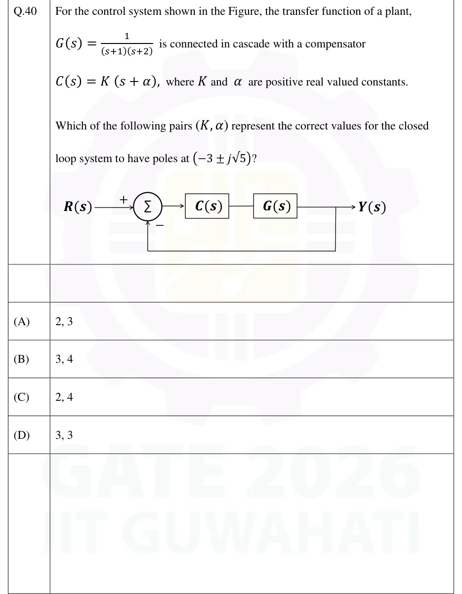
GATE 2026 EC question 40: Unity negative feedback block diagram. — Figure from the GATE 2026 EC paper. It is part of the question.

(A)
2, 3
(B)
3, 4
(C)
2, 4
(D)
3, 3

Answer and solution

GATE 2026 EC Q.40: answer and solution

GATE 2025 EC Q.36

GATE 2025 · ECQ.36 · 2 marks · MCQ

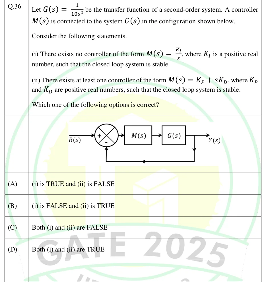
Let $G (s) = \frac{1}{10 s ^{2}}$ be the transfer function of a second-order system. A controller $M (s)$ is connected to the system $G (s)$ in the configuration shown below.

Consider the following statements.

(i) There exists no controller of the form $M (s) = \frac{K _{I}}{s}$ , where $K_{I}$ is a positive real number, such that the closed loop system is stable.

(ii) There exists at least one controller of the form $M (s) = K_{P} + s K_{D}$ , where $K_{P}$ and $K_{D}$ are positive real numbers, such that the closed loop system is stable.

Which one of the following options is correct?

GATE 2025 EC question 36: Unity negative feedback loop. — Figure from the GATE 2025 EC paper. It is part of the question.

(A)
(i) is TRUE and (ii) is FALSE
(B)
(i) is FALSE and (ii) is TRUE
(C)
Both (i) and (ii) are FALSE
(D)
Both (i) and (ii) are TRUE

Answer and solution

GATE 2025 EC Q.36: answer and solution

GATE 2025 EE Q.65

GATE 2025 · EEQ.65 · 2 marks · NAT

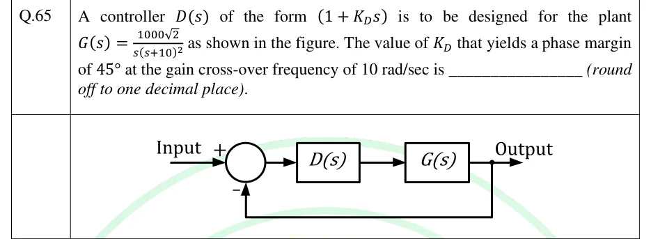
A controller $D (s)$ of the form $(1 + K_{D} s)$ is to be designed for the plant $G (s) = \frac{1000 2}{s ( s + 10 ) ^{2}}$ as shown in the figure. The value of $K_{D}$ that yields a phase margin of $4 5^{\circ}$ at the gain cross-over frequency of 10 rad/sec is ________ (round off to one decimal place).

GATE 2025 EE question 65: Unity negative feedback loop. — Figure from the GATE 2025 EE paper. It is part of the question.

Answer and solution

GATE 2025 EE Q.65: answer and solution

GATE 2025 IN Q.47

GATE 2025 · INQ.47 · 2 marks · MCQ

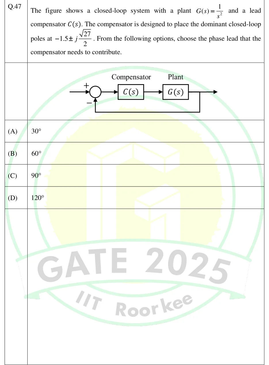
The figure shows a closed-loop system with a plant $G (s) = \frac{1}{s ^{2}}$ and a lead compensator $C (s)$ . The compensator is designed to place the dominant closed-loop poles at $- 1.5 \pm j \frac{27}{2}$ . From the following options, choose the phase lead that the compensator needs to contribute.

GATE 2025 IN question 47: Unity negative feedback loop. — Figure from the GATE 2025 IN paper. It is part of the question.

(A)
$3 0^{\circ}$
(B)
$6 0^{\circ}$
(C)
$9 0^{\circ}$
(D)
$12 0^{\circ}$

Answer and solution

GATE 2025 IN Q.47: answer and solution

GATE 2025 IN Q.50

GATE 2025 · INQ.50 · 2 marks · MSQ

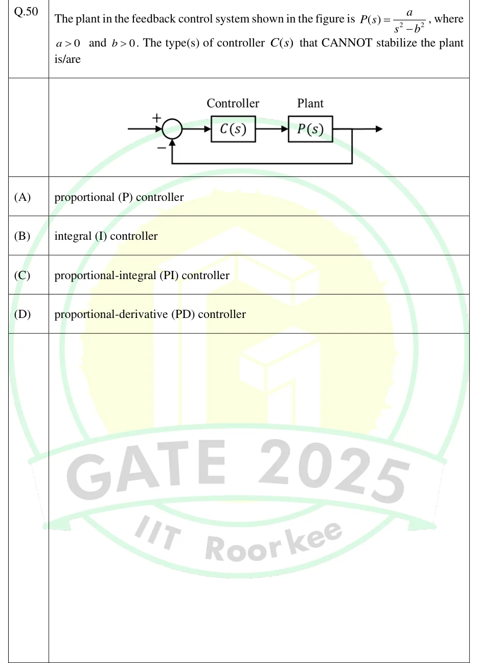
The plant in the feedback control system shown in the figure is $P (s) = \frac{a}{s ^{2} - b ^{2}}$ , where $a > 0$ and $b > 0$ . The type(s) of controller $C (s)$ that CANNOT stabilize the plant is/are

GATE 2025 IN question 50: Unity negative feedback loop. — Figure from the GATE 2025 IN paper. It is part of the question.

(A)
proportional (P) controller
(B)
integral (I) controller
(C)
proportional-integral (PI) controller
(D)
proportional-derivative (PD) controller

Answer and solution

GATE 2025 IN Q.50: answer and solution

GATE 2024 EC Q.38

GATE 2024 · ECQ.38 · 2 marks · MCQ

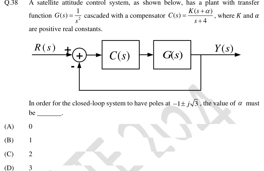
A satellite attitude control system, as shown below, has a plant with transfer function $G (s) = \frac{1}{s ^{2}}$ cascaded with a compensator $C (s) = \frac{K ( s + α )}{s + 4}$ , where $K$ and $α$ are positive real constants.

[Figure: unity negative feedback loop with $C (s)$ and $G (s)$ in cascade]

In order for the closed-loop system to have poles at $- 1 \pm j 3$ , the value of $α$ must be ________.

GATE 2024 EC question 38: Block diagram: input R(s) enters a summing junction with sign + on the reference input and sign - on the feedback input. — Figure from the GATE 2024 EC paper. It is part of the question.

(A)
0
(B)
1
(C)
2
(D)
3

Answer and solution

GATE 2024 EC Q.38: answer and solution

GATE 2023 EE Q.14

GATE 2023 · EEQ.14 · 1 mark · MCQ

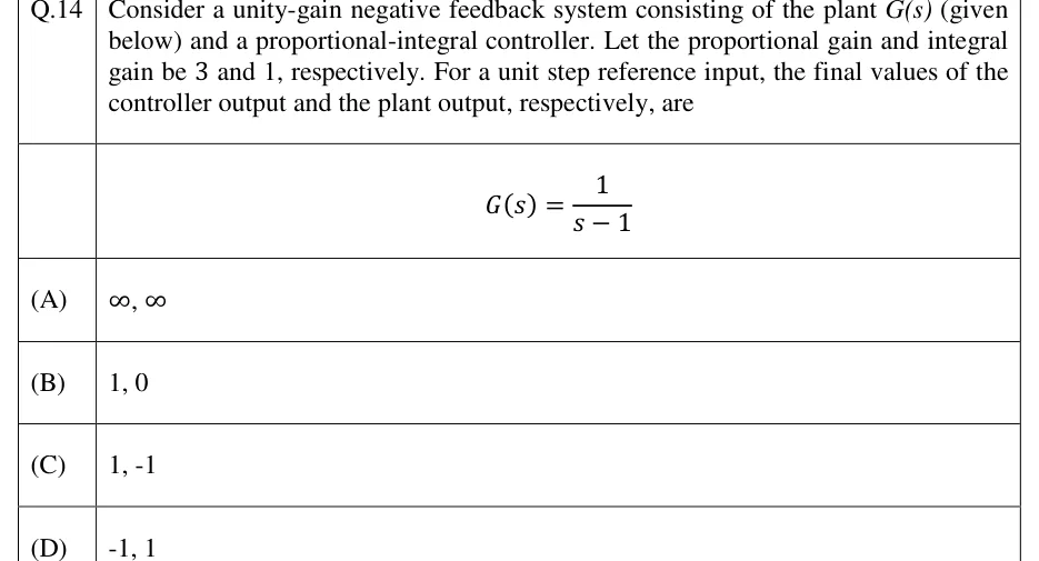
Consider a unity-gain negative feedback system consisting of the plant $G (s)$ (given below) and a proportional-integral controller. Let the proportional gain and integral gain be 3 and 1, respectively. For a unit step reference input, the final values of the controller output and the plant output, respectively, are

G (s) = \frac{1}{s - 1}

(A)
$\infty, \infty$
(B)
$1, 0$
(C)
$1, - 1$
(D)
$- 1, 1$

Answer and solution

GATE 2023 EE Q.14: answer and solution

See the question in the paper

Tap to open full size

GATE 2023 EE Q.14: answer and solution

GATE 2023 EE Q.38

GATE 2023 · EEQ.38 · 2 marks · MCQ

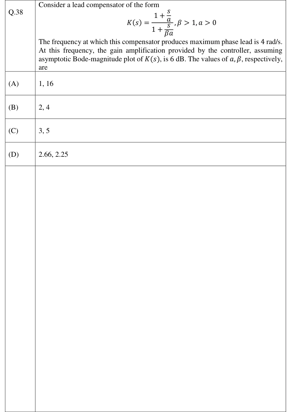
Consider a lead compensator of the form

K (s) = \frac{1 + \frac{s}{a}}{1 + \frac{s}{β a}}, β > 1, a > 0

The frequency at which this compensator produces maximum phase lead is 4 rad/s. At this frequency, the gain amplification provided by the controller, assuming asymptotic Bode-magnitude plot of $K (s)$ , is 6 dB. The values of $a, β$ , respectively, are

(A)
1, 16
(B)
2, 4
(C)
3, 5
(D)
2.66, 2.25

Answer and solution

GATE 2023 EE Q.38: answer and solution

See the question in the paper

Tap to open full size

GATE 2023 EE Q.38: answer and solution

GATE 2023 IN Q.48

GATE 2023 · INQ.48 · 2 marks · NAT

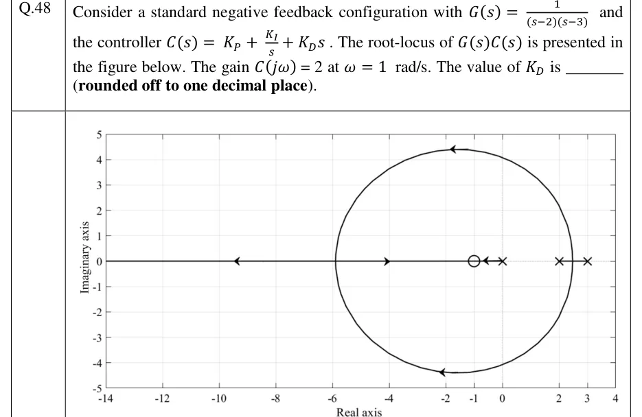
Consider a standard negative feedback configuration with $G (s) = \frac{1}{( s - 2 ) ( s - 3 )}$ and the controller $C (s) = K_{P} + \frac{K _{I}}{s} + K_{D} s$ . The root-locus of $G (s) C (s)$ is presented in the figure below. The gain $C (j ω) = 2$ at $ω = 1$ rad/s. The value of $K_{D}$ is ______ (rounded off to one decimal place).

GATE 2023 IN question 48: Root-locus plot. — Figure from the GATE 2023 IN paper. It is part of the question.

Answer and solution

GATE 2023 IN Q.48: answer and solution

GATE 2020 IN Q.6

GATE 2020 · INQ.6 · 1 mark · MCQ

A phase lead network has the transfer function $G (s) = \frac{1 + 0.2 s}{1 + 0.05 s}$ . The angular frequency at which the maximum phase shift for the network occurs is ____

(A)
10 rad/s
(B)
20 rad/s
(C)
100 rad/s
(D)
200 rad/s

Answer and solution

GATE 2020 IN Q.6: answer and solution

See the question in the paper

Tap to open full size

GATE 2020 IN Q.6: answer and solution

PRACTICE

6 questions to test yourself

PRACTICE 11 mark · NAT

A cascade compensator has transfer function $G_{c} (s) = \frac{1 + 0.9 s}{1 + 0.1 s}$ . The maximum phase lead it provides, in degrees, is ______ (round off to two decimal places).

Answer and solution

Answer: $53.13$ (accepted range $\pm 0.1$ )

Compare with $\frac{1 + a T s}{1 + T s}$ : $T = 0.1$ s and $a T = 0.9$ s, so $a = 9$ . The zero is at $- 1.11$ and the pole at $- 10$ , so it is a lead.
$sin ϕ_{m} = \frac{a - 1}{a + 1} = \frac{8}{10} = 0.8$ .
$ϕ_{m} = sin^{- 1} (0.8) = 53.1 3^{\circ}$ , occurring at $ω_{m} = \frac{1}{T a} = \frac{1}{0.3} = 3.33$ rad/s.

PRACTICE 21 mark · MCQ

A unity-feedback system has plant $G (s) = \frac{16}{s ( s + 4 )}$ . A cascade controller $G_{c} (s) = 1 + T_{d} s$ is added. The value of $T_{d}$ (in seconds) that makes the damping ratio of the closed-loop poles equal to 0.8 is

(A)
0.075
(B)
0.15
(C)
0.30
(D)
0.40

Answer and solution

Answer: (B)

Uncompensated: $s^{2} + 4 s + 16 = 0$ , so $ω_{n} = 4$ rad/s and $ζ = \frac{4}{2 \times 4} = 0.5$ .
With $G_{c} = 1 + T_{d} s$ : $s (s + 4) + 16 (1 + T_{d} s) = s^{2} + (4 + 16 T_{d}) s + 16 = 0$ , and $ω_{n}$ stays at 4 rad/s.
$2 ζ^{'} ω_{n} = 4 + 16 T_{d}$ with $ζ^{'} = 0.8$ gives $6.4 = 4 + 16 T_{d}$ , so $T_{d} = 0.15$ s. This agrees with $ζ^{'} = ζ + ω_{n} T_{d} /2 = 0.5 + 2 T_{d}$ .
0.40 comes from ignoring the plant's own damping term; 0.075 comes from dropping the factor $\frac{1}{2}$ in $ω_{n} T_{d} /2$ .

PRACTICE 32 marks · NAT

The plant $G (s) = \frac{2}{( s + 1 ) ^{3}}$ is in a unity-feedback loop. Its ultimate gain and ultimate period are found with proportional control, and a PID controller $G_{c} (s) = K_{p} (1 + \frac{1}{T _{i} s} + T_{d} s) = K_{p} + \frac{K _{i}}{s} + K_{d} s$ is then set from the Ziegler-Nichols ultimate-gain (sustained-oscillation) table. The value of $K_{d}$ is ______ (round off to two decimal places).

Answer and solution

Answer: $1.09$ (accepted range $\pm 0.01$ )

$1 + \frac{2 K}{( s + 1 ) ^{3}} = 0$ gives $s^{3} + 3 s^{2} + 3 s + 1 + 2 K = 0$ .
The Routh $s^{1}$ row is $\frac{9 - ( 1 + 2 K )}{3}$ , which is zero at $K_{u} = 4$ . The auxiliary equation $3 s^{2} + 9 = 0$ gives $ω_{u} = 3$ rad/s, so $P_{u} = \frac{2 π}{3} = 3.628$ s. Check: the phase $- 3 tan^{- 1} ω$ reaches $- 18 0^{\circ}$ at $ω = 3$ , where $∣ G ∣ = 2/8 = 0.25$ .
Ziegler-Nichols PID: $K_{p} = 0.6 K_{u} = 2.4$ and $T_{d} = 0.125 P_{u} = 0.4534$ s.
$K_{d} = K_{p} T_{d} = 2.4 \times 0.4534 = 1.088 \approx 1.09$ , which equals $0.075 K_{u} P_{u}$ .

PRACTICE 42 marks · MCQ

The open-loop unit-step response of a process is S-shaped and settles at 1. The tangent drawn at its inflection point cuts the time axis at $t = 0.5$ s and meets the final-value line at $t = 4.5$ s. Using the Ziegler-Nichols step-response (reaction-curve) method, the PID controller $G_{c} (s) = K_{p} + \frac{K _{i}}{s} + K_{d} s$ is

(A)
$10.8 + \frac{10.8}{s} + 2.7 s$
(B)
$9.6 + \frac{19.2}{s} + 1.2 s$
(C)
$9.6 + \frac{9.6}{s} + 2.4 s$
(D)
$9.6 + \frac{4.8}{s} + 4.8 s$

Answer and solution

Answer: (C)

The tangent meets the time axis at $t = L$ , so $L = 0.5$ s. It meets the final-value line at $t = L + T = 4.5$ s, so $T = 4$ s. The process gain is $K = 1$ .
PID row: $K_{p} = 1.2 \frac{T}{K L} = 1.2 \times 8 = 9.6$ , $T_{i} = 2 L = 1$ s, $T_{d} = 0.5 L = 0.25$ s.
$K_{i} = K_{p} / T_{i} = 9.6$ and $K_{d} = K_{p} T_{d} = 2.4$ , so $G_{c} (s) = 9.6 + \frac{9.6}{s} + 2.4 s$ (option C).
Option A wrongly takes $T = 4.5$ s. Options B and D use wrong multiples of $L$ for $T_{i}$ and $T_{d}$ .

PRACTICE 52 marks · MSQ

A unity-feedback system with plant $G (s) = \frac{K}{s ( s + 4 )}$ , $K > 0$ , is compensated by the cascade network $G_{c} (s) = \frac{s + 0.2}{s + 0.02}$ . Which of the following statements is/are correct?

(A)
$G_{c} (s)$ is a lag compensator.
(B)
For the same $K$ , the velocity error constant of the compensated system is 10 times that of the uncompensated system.
(C)
The maximum phase lag of $G_{c} (j ω)$ occurs at $ω \approx 0.0632$ rad/s.
(D)
$G_{c} (j ω)$ contributes positive phase at every frequency $ω > 0$ .

Answer and solution

Answer: (A), (B), (C)

The pole at $- 0.02$ is nearer the origin than the zero at $- 0.2$ , so $G_{c}$ is a lag compensator (A correct). Its phase $tan^{- 1} \frac{ω}{0.2} - tan^{- 1} \frac{ω}{0.02}$ is negative for every $ω > 0$ (D wrong).
Uncompensated $K_{v} = lim_{s \to 0} s \frac{K}{s ( s + 4 )} = \frac{K}{4}$ . Compensated $K_{v} = \frac{0.2}{0.02} \cdot \frac{K}{4} = \frac{10 K}{4}$ , ten times larger (B correct). The compensated characteristic equation $s^{3} + 4.02 s^{2} + (K + 0.08) s + 0.2 K = 0$ passes the Routh test for every $K > 0$ , so the comparison is meaningful.
Maximum lag occurs at $ω_{m} = 0.2 \times 0.02 = 0.004 = 0.0632$ rad/s (C correct). Its size is $sin^{- 1} \frac{10 - 1}{10 + 1} = 54. 9^{\circ}$ of lag.

PRACTICE 61 mark · NAT

An ideal inverting op-amp stage has input impedance $R_{1}$ in parallel with $C_{1}$ and feedback impedance $R_{2}$ in parallel with $C_{2}$ , where $R_{1} = 100 k Ω$ , $C_{1} = 1 μ F$ , $R_{2} = 10 k Ω$ and $C_{2} = 1 μ F$ . It is followed by a unity-gain inverter. The frequency, in rad/s, at which this compensator gives its maximum phase lead is ______ (round off to two decimal places).

Answer and solution

Answer: $31.62$ (accepted range $\pm 0.05$ )

The first stage gives $- \frac{Z _{2}}{Z _{1}} = - \frac{R _{2}}{R _{1}} \cdot \frac{1 + R _{1} C _{1} s}{1 + R _{2} C _{2} s}$ and the inverter removes the sign, so $G_{c} (s) = 0.1 \cdot \frac{1 + 0.1 s}{1 + 0.01 s}$ .
$R_{1} C_{1} = 0.1$ s is larger than $R_{2} C_{2} = 0.01$ s, so the zero at $- 10$ is nearer the origin than the pole at $- 100$ : a lead with $a = 10$ .
$ω_{m}$ is the geometric mean of the corners: $ω_{m} = 10 \times 100 = 1000 = 31.62$ rad/s. The arithmetic mean, 55 rad/s, is the common wrong answer.
For reference, the maximum lead there is $sin^{- 1} \frac{9}{11} = 54.9 0^{\circ}$ , and the positive constant 0.1 does not change the phase.

OFFICIAL GATE 2027 SYLLABUS WORDING

Copied from the GATE 2027 syllabus; see all 2027 syllabi.

GATE EC

compensators, PID controller

GATE EE

Lag, Lead and Lead‐Lag compensators; P, PI and PID controllers

GATE IN

on-off, P, PI, PID … controllers, tuning of PID controllers; design of lead, lag and lead-lag compensators

Preparing in Kolkata? IAE Academy's course for GATE ECE, GATE EE or GATE IN.