GATE 2026 EC Q.41
The state and output equations for a control system are:
Which of the following expressions correctly represents the transfer function of the system with zero initial conditions?
- (A)
- (B)
- (C)
- (D)

GATE EC · EE · IN
State-space models describe an LTI system by n first-order differential equations in a state vector, and , instead of by a single input-output transfer function. Solving GATE questions on this topic comes down to a small set of mechanical skills done accurately: writing a state model from a differential equation or a transfer function, recovering , computing and the time response, applying the Kalman rank tests for controllability and observability, and using controllability to place the closed-loop poles with state feedback.
16 previous-year questions · 16 solved · 6 practice questions
The state of a dynamic system at time is the smallest set of variables that, together with the input for , completely determines how the system behaves for all . These are the state variables to . Stacked into a column they form the state vector . The number is the order of the state model. It equals the degree of the characteristic polynomial and the number of eigenvalues of counted with multiplicity. For a model built from a single th-order differential equation, it also equals the order of that equation. The transfer function can have a lower order than if a pole-zero cancellation occurs (see the section on controllability and observability).
In a lumped electrical network, is the number of independent energy-storing elements, and the natural state variables are inductor currents and capacitor voltages. These carry the stored energy and cannot change instantaneously as long as the sources are bounded (no impulses). Each loop made only of capacitors (and possibly voltage sources) reduces the count by one, because KVL fixes one capacitor voltage in that loop in terms of the others. Likewise, each cut-set made only of inductors (and possibly current sources) reduces the count by one, because KCL fixes one inductor current in terms of the others.
State variables are not unique. Any invertible linear combination of a valid set, with invertible, is another valid set, so one system has infinitely many state models. All state models related by such a change of variables have the same transfer function and the same eigenvalues; only , and change, and stays the same. (A non-minimal realisation of the same , with more states, has extra eigenvalues, so this statement is about models of the same order related by .)
STATE MODEL OF A CONTINUOUS-TIME LTI SYSTEM
states, inputs, outputs. are constant matrices because the system is time-invariant.
The four matrices
Matrix | Name | Size | What it governs |
|---|---|---|---|
system (state) matrix | internal dynamics; its eigenvalues are the characteristic roots | ||
input (control) matrix | how the inputs drive the states; enters the controllability test | ||
output matrix | which combination of states is measured; enters the observability test | ||
direct transmission (feed-through) matrix | the part of the input that reaches the output directly; entry is nonzero exactly when is biproper (numerator degree = denominator degree) |
EXAM TIP
, because as . A strictly proper (numerator degree lower than denominator degree) always gives .
From a differential equation with no derivatives of the input. Take . Choose the output and its successive derivatives as the states. These are the phase variables , , . Each state is the derivative of the one before it, and the last state equation is the ODE solved for the highest derivative.
PHASE-VARIABLE MODEL OF AN ODE (NO INPUT DERIVATIVES)
The coefficient of the highest derivative must be 1 (divide through first). The same pattern holds for any order .
When derivatives of the input appear, for example , choosing , would put into the state equation, and does not allow that. Go through the transfer function instead and use a canonical form. The forms below are written for the third-order strictly proper , and the pattern extends to any order. For the example above, , so the controllable canonical form is , , . In this model the states are not and : the output is .
CONTROLLABLE CANONICAL (PHASE-VARIABLE) FORM
The denominator must be monic. The last row of holds the negated denominator coefficients in ascending powers of , and holds the numerator coefficients in ascending powers. This form is always controllable. Some texts number the states in reverse, which puts the coefficients in the first row; is the same either way.
OBSERVABLE CANONICAL FORM (DUAL OF THE CONTROLLABLE FORM)
Convention used here: , , . This form is always observable. Reversing the state order flips rows and columns without changing .
DIAGONAL (PARALLEL) FORM: DISTINCT POLES
Only for distinct poles; the are the partial-fraction residues. The residues can sit in instead of , because only each product is fixed. Complex poles give complex entries.
JORDAN FORM: REPEATED POLE
A pole of multiplicity gives a Jordan block, with on the diagonal and 1 on the superdiagonal. With this convention ( has a 1 only in the last row of each block), the coefficient of the highest power goes in the first column of that block in . If is biproper, add its constant term as .
Procedure: transfer function to controllable canonical form
Make the denominator monic by dividing the numerator and denominator by its leading coefficient.
If the numerator degree equals the denominator degree, long-divide first: . Then , and you realise the strictly proper remainder.
Put 1s on the superdiagonal of and in its last row. Every other entry is zero.
Set .
Set from the remainder numerator, in ascending powers of .
EXAM TIP
Check the companion matrix by expanding . It must return the original denominator. Writing the last row as (descending order) is an easy slip that this check catches at once.
EXAM TIP
Make the denominator monic before you read off coefficients. For , first rewrite it as . That gives last row and , not .
Take the Laplace transform of the state model with zero initial state. This gives , so and . Before any cancellation, the denominator of every entry is , so every pole comes from an eigenvalue of .
TRANSFER FUNCTION FROM A STATE MODEL
Assumes zero initial conditions. For MIMO systems is a matrix with . The order of multiplication is fixed: , then , then .
CHARACTERISTIC EQUATION
Its roots are the eigenvalues of . Every pole of is an eigenvalue. If shares a factor with , that eigenvalue cancels and does not appear as a pole. differs from only by , so the two have the same roots.
INVERSE OF A 2×2 MATRIX
Swap the diagonal entries, negate the off-diagonal ones and divide by the determinant. You use this in nearly every 2×2 calculation.
EIGENVALUE SHORTCUTS
Holds for any square , with eigenvalues counted by multiplicity. The eigenvalues of a triangular or diagonal matrix are its diagonal entries.
SIMILARITY TRANSFORMATION
is any invertible matrix. The transformation does not change the eigenvalues, the characteristic equation, , controllability or observability. With = modal matrix (eigenvectors as columns), is diagonal. This needs linearly independent eigenvectors, which is guaranteed when the eigenvalues are distinct.
MODAL MATRIX OF A COMPANION MATRIX
For in controllable canonical (companion) form, with the coefficients in the last row, the eigenvector for is . This (a Vandermonde matrix) is invertible only when the eigenvalues are distinct.
EXAM TIP
A system has many state models but only one transfer function. If two options have different matrices with the same characteristic polynomial, and both give the same , both are valid realisations. Compare and , not the matrices entry by entry.
The unforced system has solution . The matrix is the state transition matrix (STM): it carries the state from time 0 to time . It is a matrix exponential defined by a power series. It is not the matrix of element-wise exponentials . A reliable way to compute it by hand is the inverse Laplace transform of the resolvent .
STATE TRANSITION MATRIX
Valid for any constant square . The series stops after finitely many terms if is nilpotent, e.g. gives .
Method: the STM by inverse Laplace transform
Form .
Compute , which is the characteristic polynomial, and factor it.
Write .
Split every entry into partial fractions.
Take the inverse transform of each entry. Check that before you use the result.
PROPERTIES OF THE STM
True for every constant , so is always invertible. Use and to test whether a given matrix can be an STM, and to recover from a given STM.
STMS TO RECOGNISE ON SIGHT
The third matrix has eigenvalues . The last line is the diagonalisation method: is the diagonal matrix of eigenvalues and is the modal matrix, which exists when has linearly independent eigenvectors (always the case for distinct eigenvalues).
CAYLEY-HAMILTON METHOD
Basis: the Cayley-Hamilton theorem says every square matrix satisfies its own characteristic equation, so and all higher powers reduce to combinations of . The same reduction evaluates any polynomial in , such as . For with distinct eigenvalues: , with and . For a repeated eigenvalue, the distinct-eigenvalue equations are too few; add the equation you get by differentiating with respect to : .
EXAM TIP
To test whether a matrix can be an STM, check first; it is a quick filter. A matrix can pass that check and still fail. Then take and confirm , or check . Example: equals at but is not an STM.
EXAM TIP
If the unforced responses and of a second-order system are known for two linearly independent initial states and , linearity gives , so , and then . An th-order system needs independent initial states. The response to any other initial state follows without finding .
EXAM TIP
holds for all if and only if . It does work for , because commutes with every matrix. That is why the factor splits off in the rotation-type STM above.
The complete response is the sum of two parts. The zero-input response comes from the initial state with no input. The zero-state response comes from the input with zero initial state, and is the convolution of with the input. In the -domain both parts use the same resolvent , so compute it once and reuse it.
COMPLETE SOLUTION OF THE STATE EQUATION
Initial time 0. For initial time : .
OUTPUT RESPONSE
Substitute into the output equation. The term appears instantly and has no dynamics.
SOLUTION IN THE S-DOMAIN
Often the quickest route by hand. Take the inverse transform of each entry at the end.
IMPULSE RESPONSE
Zero initial state and a unit impulse input; for .
UNIT-STEP RESPONSE AND FINAL VALUES
The first formula (unit-step input, zero initial state) needs invertible. The final values hold, for any initial state, when every eigenvalue of has a negative real part; is then automatically invertible, because 0 is not an eigenvalue. You can also get by setting : .
WORKED EXAMPLE · WORKED EXAMPLE 1: STM AND COMPLETE RESPONSE
For with and a unit step, find and for .
Form , so . The eigenvalues are and .
By the 2×2 inverse rule, .
Partial fractions: , , , .
Take the inverse transform of each entry: . Check: at this is .
Zero-input part: is the first column, .
Zero-state part: . Its inverse transform is .
Add the two parts: and .
Checks: . , as the first row of requires. , which matches with .
Answer: is the matrix in step 4. For : and .
EXAM TIP
Internal (asymptotic) stability requires every eigenvalue of to have . BIBO stability depends only on the poles of that remain after cancellation. An unstable mode that is uncontrollable or unobservable cancels out of . The system can then be BIBO stable yet internally unstable. So read the question: for internal or asymptotic stability use the eigenvalues of ; for BIBO stability use the poles of in lowest terms.
EXAM TIP
To recover an earlier state of an unforced system, run the STM backwards: . You do not need to invert a matrix numerically if you already have in closed form. Replace by .
DISCRETE-TIME STATE MODEL AND ITS SOLUTION
Here are the discrete-time matrices, and plays the role of the STM. The system is asymptotically stable exactly when every eigenvalue of has . The Kalman matrices and take the same form: full rank of the first means every state can be reached from the origin, and full rank of the second means can be recovered from the output. Sampling with a zero-order hold of period gives and , which equals when is invertible.
A system is completely state controllable if, for any initial state and any target state, some input moves the state to the target in finite time. It is completely observable if the initial state can be found uniquely from the output (and the known input) over a finite interval. Controllability asks whether the input reaches every mode. Observability asks whether every mode appears in the output. Neither property depends on , and a similarity transformation changes neither.
KALMAN CONTROLLABILITY TEST
Depends only on . For a single input, is and the system is controllable exactly when . For inputs, is and you must check its rank. Compute as .
KALMAN OBSERVABILITY TEST
Depends only on . An equivalent transposed convention is , which has the same rank. For a single output, the system is observable exactly when .
DIAGONAL-FORM TEST
Use only after transforming to a diagonal with distinct eigenvalues. A zero row of means the mode cannot be excited, and a zero column of means that mode never reaches the output. In Jordan form (one block per distinct eigenvalue), check the row of at the last row of each block and the column of at the first column of each block. The test does not apply to a diagonal with a repeated eigenvalue; see the last tip of this section.
EIGENVALUE RANK TEST (MODE BY MODE)
Equivalent to the Kalman tests. An eigenvalue at which the rank drops is the uncontrollable or unobservable mode.
Controllability versus observability
Controllability | Observability | |
|---|---|---|
Question asked | Can the input steer every state anywhere in finite time? | Can the initial state be found from the output over a finite time? |
Depends on | and only | and only |
Kalman matrix | (stacked rows) | |
Condition | ||
Diagonal form, distinct | no zero row in | no zero column in |
Form that guarantees it | controllable canonical form | observable canonical form |
Duality | controllable observable | observable controllable |
Pole-zero cancellation and minimal realisation (SISO)
If and share a factor , the mode is uncontrollable, unobservable, or both.
A SISO state model is both controllable and observable (a minimal realisation) exactly when in lowest terms has order , i.e. when there is no cancellation.
The controllable canonical form of is always controllable. It is observable exactly when and have no common factor.
The observable canonical form is always observable. It is controllable exactly when there is no common factor.
A cancellation does not tell you which property fails. Run the Kalman tests to find out.
WORKED EXAMPLE · WORKED EXAMPLE 2: A HIDDEN MODE
A system has , , , . Find , test controllability and observability, and identify any hidden mode.
, so the eigenvalues are and .
. Multiplying by picks out the second column: .
. The factor cancels, so a second-order model gives a first-order .
Controllability: , , . The system is controllable, as expected for a controllable canonical form.
Observability: , , . The rank is , so the system is not observable.
Hidden mode: for , gives , and . The mode never reaches the output.
Answer: . The system is controllable but not observable, and the mode at () is the unobservable one.
EXAM TIP
For the controllability matrix is . Stopping at gives a matrix (single input) whose rank can never reach 3. Build the matrix out to (or for observability).
EXAM TIP
For a single-input system ( square), when or contains a parameter, the roots of are exactly the parameter values that make the system uncontrollable; for a single output, the roots of are the values that make it unobservable. For a single input with , if is an eigenvector of then , the columns of are dependent, and the system is uncontrollable.
EXAM TIP
If one eigenvalue has two or more Jordan blocks, a single-input system cannot be controllable and a single-output system cannot be observable. The simplest case is with .
STATE FEEDBACK AND POLE PLACEMENT
is ( for a single input) and is the new reference input. The eigenvalues of can be placed at any chosen locations (complex ones in conjugate pairs) if and only if is controllable. In the pole-placement formula, is the desired closed-loop characteristic polynomial and . State feedback does not change controllability and, for a SISO system, does not move the zeros of the transfer function; it can destroy observability if a closed-loop pole is placed on a zero.
EXAM TIP
Shortcut in controllable canonical form: if has last row , and , then is still in that form with last row . Match coefficients with the desired polynomial: . For any other form, expand and match coefficients.
PREVIOUS-YEAR QUESTIONS
Try each question first, then open the answer. We placed each question under a topic ourselves; the exam paper does not label topics.
See these papers in full: GATE ECE 2026 · GATE ECE 2025 · GATE ECE 2024 · GATE ECE 2023 · GATE ECE 2020 · GATE ECE 2018 · GATE EE 2026 · GATE EE 2025 · GATE EE 2023 · GATE EE 2018 · GATE IN 2026 · GATE IN 2024 · GATE IN 2022 · GATE IN 2020 · GATE IN 2018
The state and output equations for a control system are:
Which of the following expressions correctly represents the transfer function of the system with zero initial conditions?
A system is characterized by the following state equation and output equation (: input, : state vector, : output)
What are the values of and for which the poles of the transfer function are at and ?
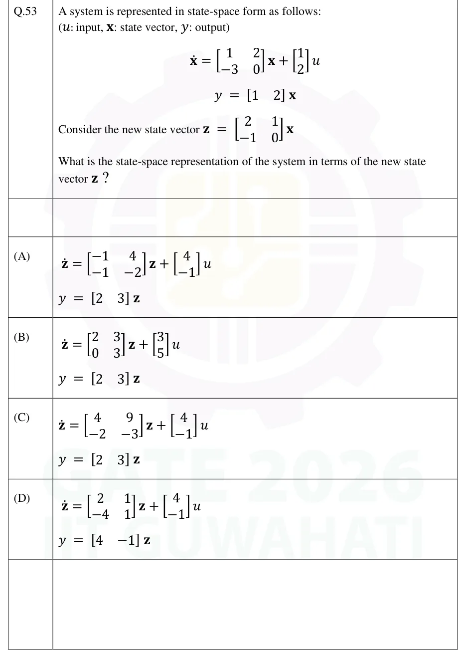
A system is represented in state-space form as follows: (: input, : state vector, : output)
Consider the new state vector
What is the state-space representation of the system in terms of the new state vector ?
,
,
,
,
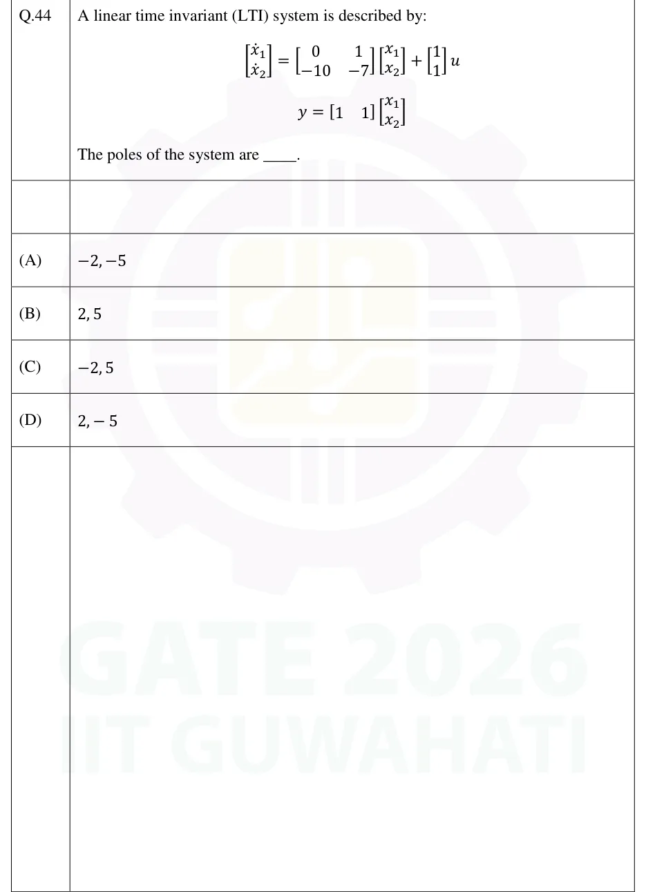
A linear time invariant (LTI) system is described by:
The poles of the system are ____.
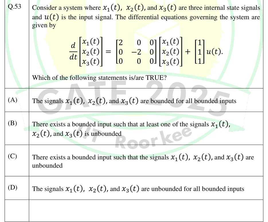
Consider a system where , and are three internal state signals and is the input signal. The differential equations governing the system are given by
Which of the following statements is/are TRUE?
The signals , and are bounded for all bounded inputs
There exists a bounded input such that at least one of the signals , and is unbounded
There exists a bounded input such that the signals , and are unbounded
The signals , and are unbounded for all bounded inputs
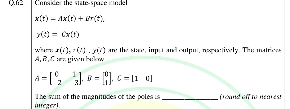
Consider the state-space model
where , , are the state, input and output, respectively. The matrices are given below
The sum of the magnitudes of the poles is ________ (round off to nearest integer).
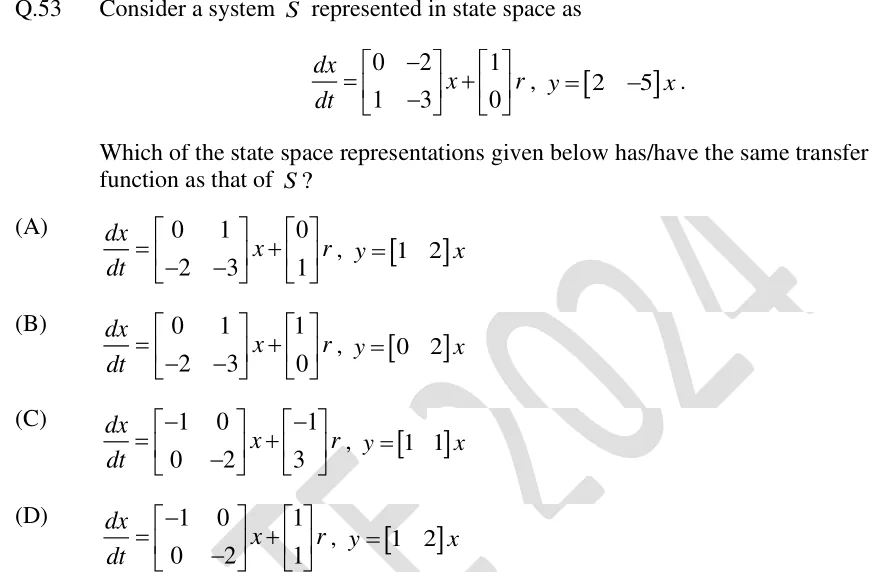
Q.53 Consider a system represented in state space as
Which of the state space representations given below has/have the same transfer function as that of ?
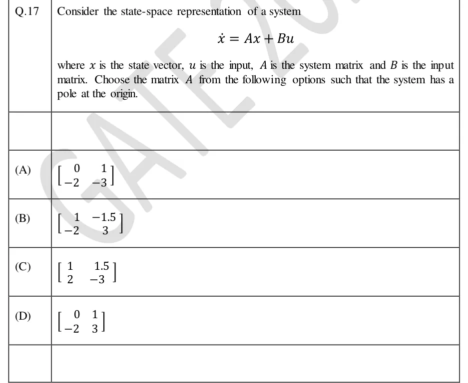
Consider the state-space representation of a system
where is the state vector, is the input, is the system matrix and is the input matrix. Choose the matrix from the following options such that the system has a pole at the origin.
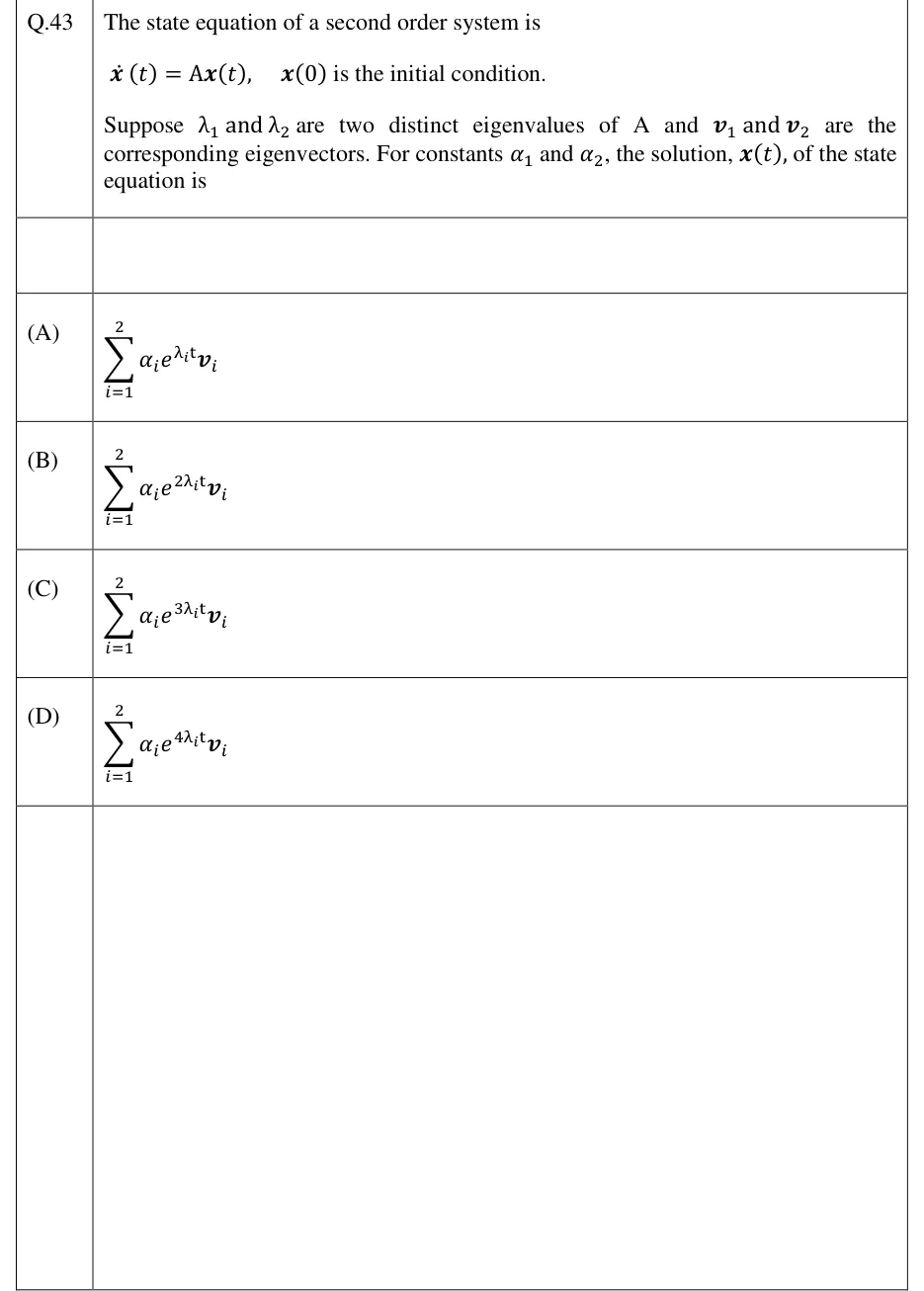
The state equation of a second order system is
Suppose and are two distinct eigenvalues of and and are the corresponding eigenvectors. For constants and , the solution, , of the state equation is
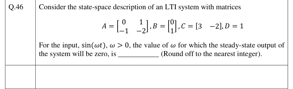
Consider the state-space description of an LTI system with matrices
For the input, , , the value of for which the steady-state output of the system will be zero, is ________ (Round off to the nearest integer).
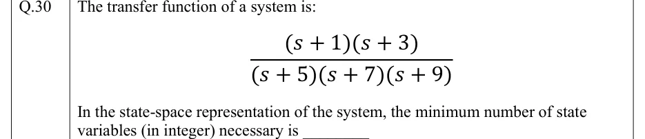
The transfer function of a system is:
In the state-space representation of the system, the minimum number of state variables (in integer) necessary is ________
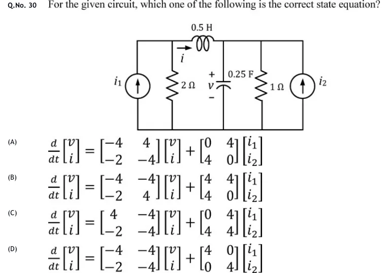
For the given circuit, which one of the following is the correct state equation?
 Tap to open full size
Two-node circuit with a common bottom (ground) rail. Left top node: an independent current source i_1 (arrow pointing up, injecting current into the left top node) and a 2 Ω resistor, both connected between the left top node and ground. The left top node connects to the right top node through a series inductor of 0.5 H in the top rail; the inductor current i is marked with an arrow flowing left to right. Right top node: a 0.25 F capacitor with voltage v (+ at top, - at bottom), a 1 Ω resistor, and an independent current source i_2 (arrow pointing up, injecting current into the right top node), all connected between the right top node and ground.
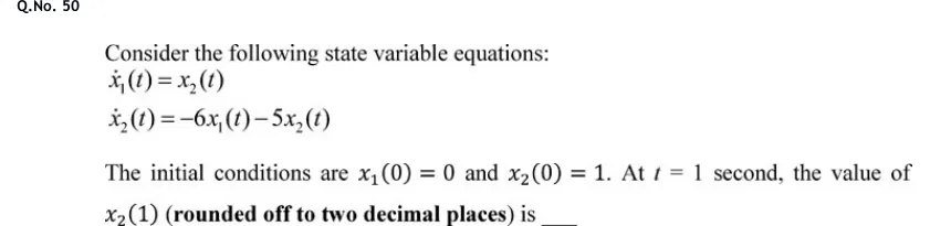
Consider the following state variable equations:
The initial conditions are and . At second, the value of (rounded off to two decimal places) is ____
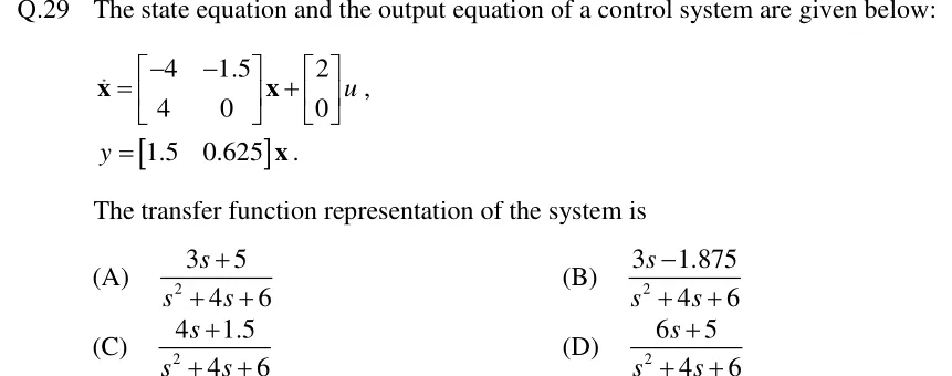
The state equation and the output equation of a control system are given below:
The transfer function representation of the system is
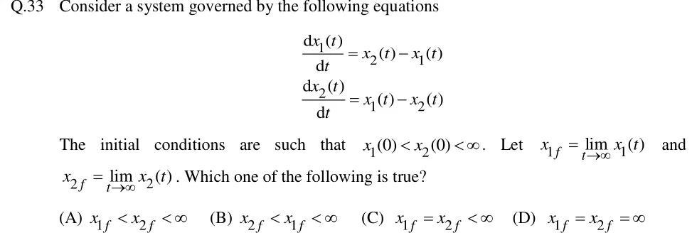
Consider a system governed by the following equations
The initial conditions are such that . Let and . Which one of the following is true?
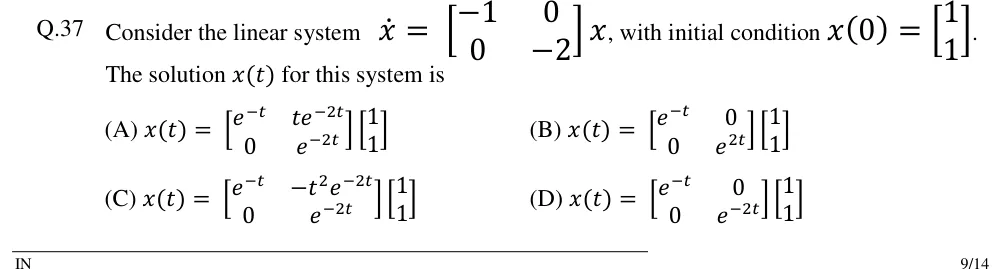
Consider the linear system , with initial condition . The solution for this system is
PRACTICE
A system is described by and . With zero initial state and a unit-step input , the steady-state value of is ______ (rounded to two decimal places).
Answer: (accepted range )
and are in controllable canonical form, so .
The eigenvalues and are in the left half-plane, so a steady state exists.
. Cross-check: , so and .
For the system , where is a real constant, the system is NOT completely state controllable if and only if
or
or
there is no real value of
Answer: (B)
.
, so .
The system is uncontrollable exactly when , i.e. or .
Why: has eigenvalues and , with eigenvectors . At these values of , is itself an eigenvector, so the input excites only one mode.
For the system , , with initial state and a unit-step input applied at , the value of at s is ______ (rounded to three decimal places).
Answer: (accepted range )
, so .
.
Zero-input part: .
Zero-state part: , so .
Total: (the terms cancel). Check: .
.
Consider an th-order LTI system , , with and state transition matrix . Which of the following statements is/are TRUE?
is invertible for every finite , and .
A change of state variables with invertible leaves the eigenvalues and the transfer function unchanged.
If has a pole-zero cancellation, the system must be uncontrollable.
for any two matrices and .
Answer: (A), (B)
A is true: , and .
B is true: , and .
C is false: a cancellation means the system is uncontrollable or unobservable. Worked example 2 has a cancellation and is controllable but unobservable.
D is false: the identity (for all ) needs .
For the system , the state feedback with places the closed-loop eigenvalues at and . The value of is ______.
Answer:
The pair is controllable (, ), so the poles can be placed anywhere.
, so .
Desired polynomial: .
Match coefficients: , and .
. Cross-check with the pole-placement formula: , , so .
Which of the following matrices can be the state transition matrix of a continuous-time LTI system , where is a constant real matrix?
Answer: (A), (B)
An STM must satisfy . Option D gives at , so it is rejected. A, B and C pass this check.
For the rest, take and check that .
A: , and . Valid (a Jordan block with ).
B: , and . Valid.
C: , and , but . Not valid. Also . The true for this is .
OFFICIAL GATE 2027 SYLLABUS WORDING
Copied from the GATE 2027 syllabus; see all 2027 syllabi.
GATE EC
State variable model and solution of state equation of LTI systems
GATE EE
State space model, Solution of state equations of LTI systems
GATE IN
state-space representation of systems
Preparing in Kolkata? IAE Academy's course for GATE ECE, GATE EE or GATE IN.