GATE EC · EE · IN

Modelling, block diagrams and signal flow graphs

This topic covers how a physical system (a circuit, a mass-spring-damper, a motor, a sensor loop) becomes a transfer function, and how a network of such transfer functions is reduced to one closed-loop transfer function using block-diagram algebra or Mason's gain formula. It also explains what negative feedback does to gain, sensitivity, disturbances, noise and bandwidth. Later Control Systems work starts from the transfer functions derived here. Time response and steady-state error use the closed-loop or error transfer function. Root locus, Bode and Nyquist analysis use the loop transfer function (the product of all the gains around the loop). An error at this stage therefore carries through to every answer that follows.

10 previous-year questions · 10 solved · 7 practice questions

1. Open loop, closed loop and the feedback principle

An open-loop system applies a control action that does not depend on the output. Examples are a heater run on a timer, or a stepper motor driven by a fixed pulse count. If the plant drifts or a disturbance arrives, nothing corrects it. A closed-loop (feedback) system measures the output with a sensor and compares that measurement with the reference. The difference (the actuating or error signal) drives the plant. With negative feedback the measured signal is subtracted at the comparator; with positive feedback it is added.

The standard single loop works like this. The reference $R (s)$ enters a comparator. The forward path $G (s)$ (controller, actuator and plant in cascade) produces the output $C (s)$ . The feedback path $H (s)$ (the sensor or transducer) returns $B (s) = H (s) C (s)$ to the comparator, and the actuating signal is $E (s) = R (s) - B (s)$ . The product of everything around the loop, $G (s) H (s)$ , is the open-loop or loop transfer function. Root locus, Bode and Nyquist analysis all work on $G (s) H (s)$ .

CLOSED-LOOP TRANSFER FUNCTION (NEGATIVE FEEDBACK)

T (s) = \frac{C ( s )}{R ( s )} = \frac{G ( s )}{1 + G ( s ) H ( s )}

Here the feedback signal is subtracted at the comparator. The characteristic equation is $1 + G (s) H (s) = 0$ . After clearing fractions, its roots are the closed-loop poles.

CLOSED-LOOP TRANSFER FUNCTION (POSITIVE FEEDBACK)

T (s) = \frac{G ( s )}{1 - G ( s ) H ( s )}

Here the feedback signal is added at the comparator. The characteristic equation is $1 - G (s) H (s) = 0$ .

ACTUATING-SIGNAL TRANSFER FUNCTION

\frac{E ( s )}{R ( s )} = \frac{1}{1 + G ( s ) H ( s )}

This uses $E = R - H C$ with negative feedback. For unity feedback ( $H = 1$ ), $E$ is the true error $R - C$ . With non-unity $H$ , the actuating signal is not the reference-minus-output error.

Role of sensing. A loop can only regulate what its sensor reports. With high loop gain ( $∣ G H ∣ ≫ 1$ ), $C / R \approx 1/ H$ . The closed-loop gain is then set almost entirely by the sensor, and the forward-path hardware barely matters. The flip side is that sensor errors are not corrected. A 2% gain error in $H$ becomes roughly a 2% error in the output. Sensor noise enters the comparator at the same point as the reference, so the loop passes it to the output instead of rejecting it. The sensor therefore has to be at least as accurate, and at least as quiet, as the output accuracy you need.

Aspect	Open loop	Closed loop (negative feedback)
Control action depends on the output?	No	Yes, through the sensor
Overall gain	$G$	$G / (1 + G H)$ , reduced by the factor $∣1 + G H ∣$
Sensitivity to a change in $G$	$S_{G}^{T} = 1$ (full)	$S_{G}^{T} = 1/ (1 + G H)$
Disturbance entering the forward path	Passes uncorrected	Reduced by the factor $∣1 + G H ∣$ compared with open loop (Section 4)
Accuracy set by	Calibration of every block	Mainly the sensor $H$ and the reference
Stability	A stable plant stays stable	Can stabilise an unstable plant or destabilise a stable one
Bandwidth	That of the plant	Generally increased
Cost and complexity	Lower	Higher (sensor and comparator needed)

Component	Role in the loop	Linear model
Potentiometer pair	Error detector for angular position	$v_{e} = K_{p} (θ_{r} - θ_{c})$ , with $K_{p}$ in V/rad
Synchro transmitter + control transformer	AC error detector for angular position	The error voltage is an amplitude-modulated (suppressed-carrier) AC signal whose amplitude is $\propto sin (θ_{r} - θ_{c}) \approx K_{s} (θ_{r} - θ_{c})$ near null
Tachogenerator	Speed sensor, used for rate (derivative) feedback	$v_{t} = K_{t g} \frac{d θ}{d t}$ , so $\frac{V _{t} ( s )}{Θ ( s )} = K_{t g} s$
DC servomotor	Actuator	Armature-controlled and field-controlled models are in Section 3
Two-phase AC servomotor	Actuator for low-power instrument servos	$\frac{Θ ( s )}{V _{c} ( s )} = \frac{K _{m}}{s ( τ _{m} s + 1 )}$ , from the linearised torque-speed curve; its negative slope acts as damping
Gear train	Matches motor speed and torque to the load	$N_{1} θ_{1} = N_{2} θ_{2}$ (Section 3)
Amplifier / controller	Shapes the actuating signal	A gain $K_{a}$ or a compensator $G_{c} (s)$

EXAM TIP

In a question, 'open-loop transfer function' normally means the loop gain $G (s) H (s)$ , not the forward path $G (s)$ alone. The two are the same only when $H = 1$ . Check which one the question gives before you form $1 + G H$ .

2. Transfer function, poles and zeros

The transfer function of a linear time-invariant (LTI) system is the Laplace transform of the output divided by the Laplace transform of the input, with all initial conditions zero. It depends only on the system, not on the input applied, and it equals the Laplace transform of the impulse response. It is not defined for nonlinear or time-varying systems. It describes only the input-output relationship: a mode cancelled between numerator and denominator is still physically present, even though the transfer function no longer shows it.

DEFINITION OF THE TRANSFER FUNCTION

G (s) = \frac{Y ( s )}{U ( s )}_{zero initial conditions} = L {g (t)}

Applies to LTI systems only. $g (t)$ is the unit-impulse response.

TRANSFER FUNCTION FROM A LINEAR DIFFERENTIAL EQUATION

a_{n} y^{(n)} + \dots + a_{1} \overset{y}{˙} + a_{0} y = b_{m} u^{(m)} + \dots + b_{1} \overset{u}{˙} + b_{0} u G (s) = \frac{Y ( s )}{U ( s )} = \frac{b _{m} s ^{m} + \dots + b _{1} s + b _{0}}{a _{n} s ^{n} + \dots + a _{1} s + a _{0}}

With all initial conditions zero, each $d^{k} / d t^{k}$ becomes $s^{k}$ . The denominator polynomial set to zero is the characteristic equation.

POLE-ZERO (ROOT-LOCUS) FORM

G (s) = K \frac{( s - z _{1} ) ( s - z _{2} ) \dots ( s - z _{m} )}{( s - p _{1} ) ( s - p _{2} ) \dots ( s - p _{n} )}

The zeros $z_{i}$ are the values of $s$ that make $G (s) = 0$ . The poles $p_{j}$ are the roots of the denominator, where $G (s) \to \infty$ . $n$ is the order of the system. $G$ is proper if $m \leq n$ and strictly proper if $m < n$ ; physical systems are proper.

TIME-CONSTANT (BODE) FORM

G (s) = \frac{K _{d c} ( 1 + s T _{1} ) ( 1 + s T _{2} ) \dots}{s ^{N} ( 1 + s τ _{1} ) ( 1 + s τ _{2} ) \dots}

$N$ is the number of poles at the origin. For the loop $G (s) H (s)$ , $N$ is the type. With $N = 0$ , $K_{d c} = G (0)$ is the DC gain, which is the steady-state output per unit step if the system is stable.

Setting the denominator to zero gives the characteristic equation. Its roots, the poles, fix the natural (transient) modes. A simple real pole at $s = - a$ contributes $e^{- a t}$ . A real pole repeated $r$ times contributes $e^{- a t}, t e^{- a t}, \dots, t^{r - 1} e^{- a t}$ . A complex pair $s = - σ \pm j ω_{d}$ contributes $e^{- σ t} sin (ω_{d} t + ϕ)$ . Zeros create no modes of their own; they only change how strongly each mode is excited. A proper rational transfer function, with common factors cancelled, is BIBO stable if and only if every pole lies strictly in the left half of the s-plane. If a right-half-plane pole is cancelled by a zero, the transfer function looks stable, but the physical system is still internally unstable. For a closed loop $T = G / (1 + G H)$ , the poles are the roots of $1 + G (s) H (s) = 0$ , not the poles of $G (s) H (s)$ . The closed-loop zeros are the zeros of $G (s)$ together with the poles of $H (s)$ , unless a common factor cancels.

EXAM TIP

Read gains carefully. $G (s) = \frac{10 ( s + 2 )}{( s + 5 ) ( s + 10 )}$ has pole-zero gain $K = 10$ , but its DC gain is $G (0) = \frac{10 \times 2}{5 \times 10} = 0.4$ . Root locus uses $K$ from the pole-zero form. Bode plots and steady-state error use the time-constant form, here $\frac{0.4 ( 1 + s /2 )}{( 1 + s /5 ) ( 1 + s /10 )}$ .

EXAM TIP

Order and type are different counts. Order is the number of poles (the degree of the denominator) of the transfer function in question. Type is the number of poles at $s = 0$ of the open-loop $G (s) H (s)$ . For example, $G (s) H (s) = \frac{5}{s ( s + 1 ) ( s + 4 )}$ is third order and type 1.

EXAM TIP

If you are given the unit-step response $c (t)$ of an LTI system that starts at rest, then $G (s) = s C (s)$ and the impulse response is $g (t) = d c / d t$ (this includes an impulse if $c (t)$ jumps at $t = 0$ ). Example: $c (t) = 1 - e^{- 2 t}$ for $t \geq 0$ gives $C (s) = \frac{1}{s} - \frac{1}{s + 2} = \frac{2}{s ( s + 2 )}$ , so $G (s) = \frac{2}{s + 2}$ .

3. Mathematical modelling: electrical, mechanical and electromechanical systems

To model a physical system:

1. Choose variables: a displacement for every independently moving mass or inertia, and a current for every mesh or a voltage for every node.
2. Write the element laws.
3. Apply Newton's second law to each mass: the net applied force equals mass times acceleration. D'Alembert's principle is the same law written as a force balance that includes the inertial force $- M \overset{x}{¨}$ . For circuits, apply KVL or KCL instead.
4. Take Laplace transforms with zero initial conditions.
5. Eliminate the internal variables to get output/input.

Element	Law	Laplace form (zero initial conditions)
Mass $M$	$f = M \frac{d ^{2} x}{d t ^{2}}$	$F = M s^{2} X$
Translational damper $B$	$f = B \frac{d}{d t} (x_{1} - x_{2})$	$F = B s (X_{1} - X_{2})$
Translational spring $K$	$f = K (x_{1} - x_{2})$	$F = K (X_{1} - X_{2})$
Moment of inertia $J$	$T = J \frac{d ^{2} θ}{d t ^{2}}$	$T = J s^{2} Θ$
Rotational damper $B$	$T = B \frac{d}{d t} (θ_{1} - θ_{2})$	$T = B s (Θ_{1} - Θ_{2})$
Torsional spring $K$	$T = K (θ_{1} - θ_{2})$	$T = K (Θ_{1} - Θ_{2})$
Resistor $R$	$v = R i$	$V = R I$
Inductor $L$	$v = L \frac{d i}{d t}$	$V = s L I$
Capacitor $C$	$v = \frac{1}{C} \int i d t$	$V = \frac{I}{s C}$

Translational	Rotational	Force-voltage (F-V, loop)	Force-current (F-I, node)
Force $f$	Torque $T$	Voltage $v$	Current $i$
Mass $M$	Inertia $J$	Inductance $L$	Capacitance $C$
Damping $B$	Damping $B$	Resistance $R$	Conductance $1/ R$
Stiffness $K$	Stiffness $K$	Elastance $1/ C$	Reciprocal inductance $1/ L$
Displacement $x$	Angle $θ$	Charge $q$	Flux linkage $ψ$
Velocity $u = d x / d t$	Angular velocity $ω$	Current $i$	Voltage $v$
Elements sharing one velocity	Elements sharing one angular velocity	Carry the same current: in series, in one mesh	Share the same voltage: in parallel, across one node

MASS-SPRING-DAMPER

\frac{X ( s )}{F ( s )} = \frac{1}{M s ^{2} + B s + K}

Derived from $M \frac{d ^{2} x}{d t ^{2}} + B \frac{d x}{d t} + K x = f$ . The natural frequency is $ω_{n} = K / M$ , the damping ratio is $ζ = \frac{B}{2 K M}$ , and the DC gain (static compliance) is $1/ K$ .

ANALOGOUS CIRCUIT EQUATIONS

F-V: L \frac{d ^{2} q}{d t ^{2}} + R \frac{d q}{d t} + \frac{q}{C} = v F-I: C \frac{d v}{d t} + \frac{v}{R} + \frac{1}{L} \int v d t = i

These are the mass-spring-damper equation rewritten with the analogues. F-V gives a series RLC driven by a voltage source, with $q \leftrightarrow x$ . F-I gives a parallel RLC driven by a current source, with node voltage $v \leftrightarrow$ velocity.

SERIES RLC, OUTPUT ACROSS C

\frac{V _{C} ( s )}{V _{i} ( s )} = \frac{1}{L C s ^{2} + R C s + 1}

Series $R$ , $L$ and $C$ driven by $v_{i}$ . Here $ω_{n} = 1/ L C$ and $ζ = \frac{R}{2} C / L$ .

INVERTING OP-AMP STAGE

\frac{V _{o} ( s )}{V _{i} ( s )} = - \frac{Z _{f} ( s )}{Z _{i} ( s )}

This assumes an ideal op-amp (infinite open-loop gain, zero input current) with its non-inverting input grounded. $Z_{i}$ is in series with the input and $Z_{f}$ connects the output to the inverting input. With $Z_{i} = R_{1}$ and $Z_{f} = 1/ (s C)$ the stage is an integrator, $- 1/ (s R_{1} C)$ . A second inverting stage restores the sign. An ideal op-amp has zero output impedance, so cascaded stages do not load each other.

ARMATURE-CONTROLLED DC MOTOR

\frac{Θ ( s )}{V _{a} ( s )} = \frac{K _{t}}{s [ ( R _{a} + s L _{a} ) ( J s + B ) + K _{t} K _{b} ]}

Motor torque is $T_{m} = K_{t} i_{a}$ and back emf is $e_{b} = K_{b} d θ / d t$ , with $J$ and $B$ referred to the motor shaft. The back emf is a built-in negative velocity feedback. In SI units, $K_{t} = K_{b}$ numerically. For speed output, drop the factor $s$ : $Ω/ V_{a} = K_{t} / [(R_{a} + s L_{a}) (J s + B) + K_{t} K_{b}]$ . With a load torque $T_{L}$ opposing the motor, superposition gives $Ω (s) = \frac{K _{t} V _{a} ( s ) - ( R _{a} + s L _{a} ) T _{L} ( s )}{( R _{a} + s L _{a} ) ( J s + B ) + K _{t} K _{b}}$ .

DC MOTOR SPEED WITH NEGLIGIBLE ARMATURE INDUCTANCE

\frac{Ω ( s )}{V _{a} ( s )} = \frac{K _{m}}{τ _{m} s + 1}, K_{m} = \frac{K _{t}}{R _{a} B + K _{t} K _{b}}, τ_{m} = \frac{R _{a} J}{R _{a} B + K _{t} K _{b}}

Valid when $L_{a} \approx 0$ . $K_{m}$ is the steady-state speed per volt. The inertia $J$ affects only the time constant, not the final speed.

FIELD-CONTROLLED DC MOTOR

\frac{Θ ( s )}{V _{f} ( s )} = \frac{K _{t f}}{s ( R _{f} + s L _{f} ) ( J s + B )}

The armature current is held constant, so the torque is $T_{m} = K_{t f} i_{f}$ , where $K_{t f}$ includes that constant armature current. Back emf does not affect the torque, so, unlike the armature-controlled motor, there is no inherent velocity feedback.

GEAR TRAIN AND REFLECTED LOAD

\frac{θ _{2}}{θ _{1}} = \frac{N _{1}}{N _{2}}, J_{e q} = J_{1} + (\frac{N _{1}}{N _{2}})^{2} J_{2}, B_{e q} = B_{1} + (\frac{N _{1}}{N _{2}})^{2} B_{2}

Gear 1 (motor side) has $N_{1}$ teeth and gear 2 (load side) has $N_{2}$ . To refer a load-side $J_{2}$ , $B_{2}$ or stiffness to the motor side, multiply by $(N_{1} / N_{2})^{2}$ . For ideal lossless gears the torque scales as $T_{2} = (N_{2} / N_{1}) T_{1}$ , so a load torque $T_{L}$ referred to the motor side becomes $(N_{1} / N_{2}) T_{L}$ .

EXAM TIP

The F-I analogy keeps the mechanical layout. Every point with its own displacement (every mass) becomes one electrical node, and each mass becomes a capacitor from that node to ground. A spring or damper between two points becomes an inductor or a resistor between the corresponding nodes. A spring or damper attached to a fixed wall goes from its node to ground, because the wall is the reference node. An applied force becomes a current source into its node. The F-V analogy puts the same elements into meshes, so its circuit is the dual. Mass is analogous to inductance in F-V and to capacitance in F-I; do not mix the two columns.

WORKED EXAMPLE

Mass $M_{1}$ is driven by a force $f (t)$ and is joined to mass $M_{2}$ by a spring of stiffness $K$ . Mass $M_{2}$ is connected to a fixed wall by a viscous damper $B$ . Both masses slide without friction. Find $X_{2} (s) / F (s)$ , where $x_{2}$ is the displacement of $M_{2}$ , and describe the force-current analogue.

Solution

Newton's law on $M_{1}$ : $M_{1} \overset{x}{¨}_{1} = f - K (x_{1} - x_{2})$ . With zero initial conditions: $(M_{1} s^{2} + K) X_{1} - K X_{2} = F$ .
On $M_{2}$ : $M_{2} \overset{x}{¨}_{2} = K (x_{1} - x_{2}) - B \overset{x}{˙}_{2}$ , which gives $- K X_{1} + (M_{2} s^{2} + B s + K) X_{2} = 0$ .
From the second equation, $X_{1} = \frac{M _{2} s ^{2} + B s + K}{K} X_{2}$ . Substituting into the first: $X_{2} [(M_{1} s^{2} + K) (M_{2} s^{2} + B s + K) - K^{2}] = K F$ .
Expand; the $K^{2}$ terms cancel: $\frac{X _{2} ( s )}{F ( s )} = \frac{K}{s [ M _{1} M _{2} s ^{3} + M _{1} B s ^{2} + K ( M _{1} + M _{2} ) s + B K ]}$ .
Physical check: only the damper ties the masses to the wall, so a constant force $F_{0}$ produces a steady velocity, not a steady position. The pole at $s = 0$ shows this. The cubic factor has all its roots in the left half-plane for any positive values: all coefficients are positive, and $M_{1} B \cdot K (M_{1} + M_{2}) > M_{1} M_{2} \cdot B K$ . So the final value theorem applies to the velocity $s X_{2}$ . It gives $v_{2} (\infty) = lim_{s \to 0} \frac{K F _{0}}{M _{1} M _{2} s ^{3} + M _{1} B s ^{2} + K ( M _{1} + M _{2} ) s + B K} = \frac{F _{0}}{B}$ , which is the speed at which the damper force balances the applied force.
Force-current analogue: node 1 carries the velocity of $M_{1}$ and node 2 the velocity of $M_{2}$ . A current source $f$ feeds node 1. A capacitor $C_{1} = M_{1}$ runs from node 1 to ground. An inductor with $1/ L = K$ joins nodes 1 and 2. A capacitor $C_{2} = M_{2}$ runs from node 2 to ground. A resistor with conductance $1/ R = B$ runs from node 2 to ground, because the wall is ground.

Answer: $\frac{X _{2} ( s )}{F ( s )} = \frac{K}{s [ M _{1} M _{2} s ^{3} + M _{1} B s ^{2} + K ( M _{1} + M _{2} ) s + B K ]}$ , and a constant force $F_{0}$ gives a final velocity of $F_{0} / B$ .

4. Effects of feedback: gain, sensitivity, disturbance, noise and bandwidth

Split the forward path as $G = G_{1} G_{2}$ . A disturbance $D (s)$ is added between $G_{1}$ and $G_{2}$ . Sensor noise $N (s)$ is added to the sensor output, so the comparator forms $E = R - (H C + N)$ . By superposition, the output is:

OUTPUT WITH REFERENCE, DISTURBANCE AND SENSOR NOISE

C (s) = \frac{G _{1} G _{2}}{1 + G _{1} G _{2} H} [R (s) - N (s)] + \frac{G _{2}}{1 + G _{1} G _{2} H} D (s)

Negative feedback. The noise term has the same transfer function as the reference, with a minus sign, so no amount of loop gain can separate the two.

SENSITIVITY (DEFINITION)

S_{G}^{T} = \frac{\partial T / T}{\partial G / G} = \frac{G}{T} \frac{\partial T}{\partial G}

The fractional change in $T$ per fractional change in the parameter $G$ , equal to $\partial ln T / \partial ln G$ . It is valid for small changes. For a large change, compute $T$ before and after instead.

CLOSED-LOOP SENSITIVITY TO G AND TO H

S_{G}^{T} = \frac{1}{1 + G H}, S_{H}^{T} = \frac{- G H}{1 + G H}

For negative feedback, $T = G / (1 + G H)$ . An open loop ( $T = G$ ) has $S_{G}^{T} = 1$ . When $∣ G H ∣ ≫ 1$ , $S_{G}^{T} \to 0$ but $S_{H}^{T} \to - 1$ , so a feedback-path error reaches the output almost one-for-one. For the frequency-dependent sensitivity, evaluate at $s = j ω$ .

CHAIN RULE FOR A PARAMETER INSIDE G

S_{α}^{T} = S_{G}^{T} S_{α}^{G}

For any parameter $α$ inside $G$ . If $G = K G_{0} (s)$ , then $S_{K}^{G} = 1$ , so $S_{K}^{T} = S_{G}^{T}$ .

DISTURBANCE TRANSFER FUNCTION

\frac{C ( s )}{D ( s )} = \frac{G _{2}}{1 + G _{1} G _{2} H} \approx \frac{1}{G _{1} H} (∣ G_{1} G_{2} H ∣ ≫ 1)

For a disturbance entering after $G_{1}$ . Compared with open loop, where $C / D = G_{2}$ , feedback reduces the disturbance's effect by the factor $∣1 + G_{1} G_{2} H ∣$ . In the high-gain limit, only the gain upstream of the disturbance point (and $H$ ) sets the residual effect $1/ (G_{1} H)$ ; raising $G_{2}$ does not reduce it. For a disturbance added directly at the output, $C / D = 1/ (1 + G H)$ .

GAIN-BANDWIDTH TRADE (FIRST-ORDER PLANT)

T (s) = \frac{K}{1 + K H} \cdot \frac{1}{1 + s \frac{τ}{1 + K H}}

Plant $K / (1 + s τ)$ with a constant negative-feedback gain $H$ (use $H = 1$ for unity feedback). The DC gain falls by the factor $(1 + K H)$ . The bandwidth rises from $1/ τ$ to $(1 + K H) / τ$ rad/s, and the time constant shrinks by the same factor. The gain-bandwidth product stays $K / τ$ .

What negative feedback does (at frequencies where |1 + GH| > 1)

Reduces the overall gain by the factor $∣1 + G H ∣$ . This is the price paid for every benefit below.
Reduces the sensitivity to forward-path variations by the same factor.
Increases the bandwidth and speeds up the response (by $1 + K H$ in the first-order case).
Reduces the effect of disturbances that enter the forward path.
Does NOT reduce the sensitivity to the feedback element, and does NOT reject sensor noise.
Moves the closed-loop poles, so it can stabilise an unstable plant, or destabilise a stable one if the loop gain or phase lag is too large.
Positive feedback, $G / (1 - G H)$ , has $S_{G}^{T} = 1/ (1 - G H)$ . For real $0 < G H < 1$ , it raises both the gain and the sensitivity above their open-loop values. It is used in regenerative circuits and oscillators, not for regulation.

WORKED EXAMPLE

An amplifier has open-loop gain $G (s) = \frac{1000}{1 + s /100}$ and is placed in a negative-feedback loop with constant feedback gain $H = 0.049$ . (a) Find the closed-loop DC gain and the sensitivity of that DC gain to $G$ . (b) The amplifier's DC gain drops by 20%. Estimate the change in closed-loop DC gain from the sensitivity, then compute it exactly. (c) Compare the open-loop and closed-loop bandwidths.

Solution

DC loop gain: $G (0) H = 1000 \times 0.049 = 49$ . So $T (0) = \frac{1000}{1 + 49} = 20$ .
$S_{G}^{T} = \frac{1}{1 + G H} = \frac{1}{50} = 0.02$ .
Estimate: $\frac{Δ T}{T} \approx S_{G}^{T} \frac{Δ G}{G} = 0.02 \times (- 20%) = - 0.4%$ .
Exact: with $G = 800$ , $T = \frac{800}{1 + 39.2} = 19.90$ , a change of $- 0.50%$ . The sensitivity estimate is a small-change (first-order) approximation. Both results show a 20% drift reduced to well under 1%.
Closed loop: $T (s) = \frac{1000}{1 + s /100 + 49} = \frac{20}{1 + s /5000}$ .
Bandwidth: 100 rad/s open loop and 5000 rad/s closed loop, larger by the factor $1 + K H = 50$ . Gain times bandwidth is $1000 \times 100 = 20 \times 5000 = 1 0^{5}$ rad/s in both cases, so it is unchanged.

Answer: (a) $T (0) = 20$ and $S_{G}^{T} = 0.02$ . (b) About $- 0.4%$ estimated and $- 0.50%$ exact ( $T \approx 19.90$ ). (c) The bandwidth rises from 100 rad/s to 5000 rad/s, and the gain-bandwidth product stays $1 0^{5}$ rad/s.

EXAM TIP

The benefits of negative feedback hold only at frequencies where $∣1 + G (j ω) H (j ω) ∣ > 1$ . Where $∣1 + G H ∣ < 1$ , which can happen near gain crossover in a lightly damped loop, negative feedback increases sensitivity and amplifies disturbances instead.

EXAM TIP

Sensitivity is a derivative, so it is accurate only for small changes. In a '20% change' question with options close together, compute $T$ exactly at the new parameter value rather than using $S \times 20%$ .

5. Block diagram reduction

A block diagram shows signals (arrows) and transfer functions (blocks). A block multiplies the signal passing through it. A summing point adds or subtracts its incoming signals, each with its own sign. A takeoff (pickoff) point copies a signal to several destinations without changing it. Reduction replaces part of the diagram with an equivalent that gives the same outputs for the same inputs.

Operation	Original	Equivalent
Cascade (series) blocks	$X \to G_{1} \to G_{2} \to Y$	One block $G_{1} G_{2}$
Parallel blocks	$G_{1}$ and $G_{2}$ fed by the same $X$ , outputs summed with signs	One block $G_{1} \pm G_{2}$
Eliminate a feedback loop	Forward path $G$ , feedback path $H$	$\frac{G}{1 \pm G H}$ ( $+$ for negative feedback)
Move a summing point downstream past $G$	$(X_{1} \pm X_{2})$ enters $G$	$G X_{1} \pm G X_{2}$ : insert $G$ in the $X_{2}$ branch
Move a summing point upstream past $G$	$G X_{1} \pm X_{2}$	$G (X_{1} \pm X_{2} / G)$ : insert $1/ G$ in the $X_{2}$ branch
Move a takeoff point downstream past $G$	$X$ tapped before $G$	Tap after $G$ and insert $1/ G$ in the tapped branch
Move a takeoff point upstream past $G$	$GX$ tapped after $G$	Tap before $G$ and insert $G$ in the tapped branch
Adjacent summing points	Two summing points in a row	Interchange or merge freely
Adjacent takeoff points	Two takeoff points on one line	Interchange freely
Non-unity to unity feedback	$G$ with feedback $H$	$1/ H$ in cascade with a unity loop around $G H$

Reduction procedure

With several inputs, find the output for one input at a time with the others set to zero (superposition), then add the results. If the input you keep enters a summing point with a minus sign, carry that sign as a gain of $- 1$ .
Combine every cascade and every parallel group.
Eliminate inner loops that do not overlap other loops, innermost first.
Where loops overlap, move a summing point or takeoff point past a block to separate them, inserting the compensating block.
Repeat until a single block remains.
Cross-check: once the result is written in terms of the individual block gains, its denominator should equal $Δ$ from Mason's formula (Section 6), unless a common factor has cancelled.

EQUIVALENT UNITY-FEEDBACK FORWARD PATH

G_{e q} (s) = \frac{G ( s )}{1 + G ( s ) H ( s ) - G ( s )}

A unity negative-feedback loop around $G_{e q}$ has the same closed-loop transfer function $G / (1 + G H)$ . Use it when a steady-state-error formula assumes unity feedback, so that $E = R - C$ is the true error.

WORKED EXAMPLE

A block diagram has the forward chain $R \to S_{1} \to G_{1} \to S_{2} \to G_{2} \to A \to G_{3} \to C$ . $S_{1}$ and $S_{2}$ are summing points, and $A$ is a takeoff point on the output of $G_{2}$ . $S_{1}$ forms $R - H_{1} A - C$ : the signal at $A$ is fed back through $H_{1}$ , there is unity feedback from $C$ , and both are subtracted. $S_{2}$ forms (output of $G_{1}$ ) $- H_{2} C$ . Find $C (s) / R (s)$ by block-diagram reduction, and check it with Mason's formula.

Solution

The $H_{1}$ loop (through $G_{1}$ and $G_{2}$ ) and the $H_{2}$ loop (through $G_{2}$ and $G_{3}$ ) overlap. Each contains a block the other lacks, so neither can be eliminated first.
Move takeoff point $A$ downstream past $G_{3}$ . The fed-back signal must stay $H_{1} A = H_{1} C / G_{3}$ , so insert $1/ G_{3}$ : the branch from $C$ to $S_{1}$ now has gain $H_{1} / G_{3}$ .
The $H_{2}$ loop is now self-contained. $G_{2} G_{3}$ with feedback $H_{2}$ reduces to $\frac{G _{2} G _{3}}{1 + G _{2} G _{3} H _{2}}$ .
At $S_{1}$ , two signals taken from $C$ are both subtracted: $C$ itself and $(H_{1} / G_{3}) C$ . They are parallel feedback paths, so combine them into one feedback block $1 + H_{1} / G_{3}$ .
The forward path is now $\frac{G _{1} G _{2} G _{3}}{1 + G _{2} G _{3} H _{2}}$ . Closing the loop: $T = \frac{\frac{G _{1} G _{2} G _{3}}{1 + G _{2} G _{3} H _{2}}}{1 + \frac{G _{1} G _{2} G _{3}}{1 + G _{2} G _{3} H _{2}} ( 1 + \frac{H _{1}}{G _{3}} )} = \frac{G _{1} G _{2} G _{3}}{1 + G _{2} G _{3} H _{2} + G _{1} G _{2} G _{3} + G _{1} G _{2} H _{1}}$ .
Mason check: there is one forward path, $P_{1} = G_{1} G_{2} G_{3}$ . The loops are $L_{1} = - G_{1} G_{2} H_{1}$ , $L_{2} = - G_{2} G_{3} H_{2}$ and $L_{3} = - G_{1} G_{2} G_{3}$ . All three pass through the output node of $S_{2}$ and through $A$ , so they touch each other and the forward path. Then $Δ = 1 + G_{1} G_{2} H_{1} + G_{2} G_{3} H_{2} + G_{1} G_{2} G_{3}$ and $Δ_{1} = 1$ , which gives the same result.
Special-case check: with every block and feedback gain equal to 1, the formula gives $1/4$ . Directly: $A = C$ , the output of $S_{1}$ is $R - 2 C$ , the output of $S_{2}$ is $R - 3 C$ , and $C = R - 3 C$ , so $C = R /4$ .

Answer: $\frac{C ( s )}{R ( s )} = \frac{G _{1} G _{2} G _{3}}{1 + G _{1} G _{2} H _{1} + G _{2} G _{3} H _{2} + G _{1} G _{2} G _{3}}$

EXAM TIP

Rule for moving a point across a block: insert whatever keeps the moved signal unchanged. Moving a summing point downstream or a takeoff point upstream: insert $G$ . Moving a summing point upstream or a takeoff point downstream: insert $1/ G$ .

EXAM TIP

A summing point and a takeoff point that sit next to each other cannot be swapped without a correction branch. After the swap, the tapped signal would include (or miss) the signal the summing point adds.

EXAM TIP

Multiplying cascaded transfer functions is valid only if the second stage does not load the first. Two identical RC low-pass sections connected directly do NOT give $1/ (R C s + 1)^{2}$ ; the correct result is $1/ (R^{2} C^{2} s^{2} + 3 R C s + 1)$ . With a unity-gain buffer between the sections, the simple product is correct.

6. Signal flow graphs and Mason's gain formula

A signal flow graph (SFG) draws a set of linear equations as nodes (the variables) joined by directed branches (the gains). A node's value is the sum of all signals entering it; the branches leaving a node do not change its value. SFGs apply only to linear systems written as cause-and-effect equations of the form $x_{j} = \sum_{k} t_{k j} x_{k}$ .

Terminology

Source (input) node: only outgoing branches. Sink (output) node: only incoming branches. Mixed node: both.
Any mixed node can be made an output by adding a unity-gain branch from it to a new sink node. A mixed node cannot be made an input node this way.
Path: a sequence of connected branches followed in the branch direction, with no node visited twice.
Forward path: a path from an input node to an output node. Its gain $P_{k}$ is the product of its branch gains.
Loop: a closed path that starts and ends at the same node, with no other node visited twice. Its gain $L_{i}$ is the product of the branch gains around it, signs included.
Self-loop: a branch from a node back to itself, gain $t$ . It counts as a loop ( $L = t$ ). Removing it divides every branch entering that node by $(1 - t)$ .
Non-touching: two loops, or a loop and a path, with no node in common.

Converting a block diagram to an SFG

Make every input, every output, every summing-point output and every takeoff point a node.
Each block becomes a branch carrying that transfer function. A direct connection becomes a branch of gain 1.
Put the summing-point sign into the branch: a signal subtracted through $H$ becomes a branch of gain $- H$ .
A summing point followed immediately by a takeoff point can share one node. A takeoff point placed before a summing point on the same line must be a separate node, joined to the summing node by a unity branch. Otherwise the tapped signal wrongly includes what the summing point added.

MASON'S GAIN FORMULA

T = \frac{\sum _{k} P _{k} Δ _{k}}{Δ}

The gain from a source node to any other node. $P_{k}$ is the gain of the $k$ -th forward path. $Δ$ is the graph determinant. $Δ_{k}$ is $Δ$ recomputed with every loop that touches the $k$ -th forward path removed.

GRAPH DETERMINANT

Δ = 1 - i \sum L_{i} + i, j \sum L_{i} L_{j} - i, j, k \sum L_{i} L_{j} L_{k} + \dots

The second sum runs over every pair of mutually non-touching loops, the third over every triple, and so on. Loop gains carry their own signs, so a negative-feedback loop ( $L = - G H$ ) adds $+ G H$ to $Δ$ . $Δ = 0$ is the characteristic equation, and $Δ$ is the same for every input-output pair in a given graph.

GAIN BETWEEN TWO NON-INPUT NODES

\frac{x _{out}}{x _{m}} = \frac{( \sum _{k} P _{k} Δ _{k} ) _{x_{in} \to x_{out}}}{( \sum _{k} P _{k} Δ _{k} ) _{x_{in} \to x_{m}}}

Mason's formula applies only from a source node. For the ratio of two internal nodes, apply it from the input to each node and divide; $Δ$ cancels.

Mason procedure

List every forward path and its gain $P_{k}$ .
List every loop and its gain $L_{i}$ , with signs. Look for loops that pass through more than one feedback branch, and for loops created by feedforward branches that start at a non-source node.
Find all pairs, triples, and so on of mutually non-touching loops.
Form $Δ$ .
For each forward path, remove every loop that shares even one node with it. What remains of $Δ$ is $Δ_{k}$ , which is often 1.
Assemble $T = \sum P_{k} Δ_{k} /Δ$ , and check a special case if you can (for example, set one feedback gain to zero).

WORKED EXAMPLE

A signal flow graph has nodes $x_{1}$ (input) to $x_{6}$ (output) and these branch gains: $x_{1} \to x_{2} = 1$ , $x_{2} \to x_{3} = 2$ , $x_{3} \to x_{4} = 3$ , $x_{4} \to x_{5} = 1$ , $x_{5} \to x_{6} = 1$ , $x_{3} \to x_{2} = - 0.5$ , $x_{5} \to x_{4} = - 1$ , $x_{5} \to x_{2} = - 0.5$ , and a feedforward branch $x_{1} \to x_{4} = 4$ . There are no other branches. Find $x_{6} / x_{1}$ .

Solution

Forward paths: $P_{1}$ is $x_{1} \to x_{2} \to x_{3} \to x_{4} \to x_{5} \to x_{6}$ , with $P_{1} = 1 \cdot 2 \cdot 3 \cdot 1 \cdot 1 = 6$ . $P_{2}$ is $x_{1} \to x_{4} \to x_{5} \to x_{6}$ , with $P_{2} = 4 \cdot 1 \cdot 1 = 4$ .
Loops: $L_{1}$ is $x_{2} \to x_{3} \to x_{2}$ , $L_{1} = 2 (- 0.5) = - 1$ . $L_{2}$ is $x_{4} \to x_{5} \to x_{4}$ , $L_{2} = 1 (- 1) = - 1$ . $L_{3}$ is $x_{2} \to x_{3} \to x_{4} \to x_{5} \to x_{2}$ , $L_{3} = 2 \cdot 3 \cdot 1 \cdot (- 0.5) = - 3$ . The feedforward branch starts at the source node, so it creates no loop.
Non-touching pairs: $L_{1}$ (nodes $x_{2}, x_{3}$ ) and $L_{2}$ (nodes $x_{4}, x_{5}$ ) share no node, so $L_{1} L_{2} = 1$ . $L_{3}$ touches both. There are no triples.
$Δ = 1 - (L_{1} + L_{2} + L_{3}) + L_{1} L_{2} = 1 - (- 5) + 1 = 7$ .
$P_{1}$ passes through every node from $x_{2}$ to $x_{5}$ , so it touches all loops and $Δ_{1} = 1$ . $P_{2}$ uses $x_{1}, x_{4}, x_{5}, x_{6}$ . It touches $L_{2}$ and $L_{3}$ but not $L_{1}$ , so $Δ_{2} = 1 - L_{1} = 2$ .
$T = \frac{P _{1} Δ _{1} + P _{2} Δ _{2}}{Δ} = \frac{6 ( 1 ) + 4 ( 2 )}{7} = \frac{14}{7} = 2$ .
Check with node equations: $x_{3} = 2 x_{2}$ and $x_{2} = x_{1} - 0.5 x_{3} - 0.5 x_{5}$ give $x_{3} = x_{1} - 0.5 x_{5}$ . Then $x_{4} = 3 x_{3} + 4 x_{1} - x_{5} = 7 x_{1} - 2.5 x_{5}$ . Since $x_{5} = x_{4}$ , $3.5 x_{5} = 7 x_{1}$ , so $x_{5} = x_{6} = 2 x_{1}$ .

Answer: $x_{6} / x_{1} = 2$ . In symbols, write $G_{1}$ for $x_{2} \to x_{3}$ , $G_{2}$ for $x_{3} \to x_{4}$ , $G_{3}$ for $x_{4} \to x_{5}$ and $G_{4}$ for the feedforward branch $x_{1} \to x_{4}$ . Write $- H_{1}$ for $x_{3} \to x_{2}$ , $- H_{2}$ for $x_{5} \to x_{4}$ and $- H_{3}$ for $x_{5} \to x_{2}$ , with the other branches unity. Then $\frac{x _{6}}{x _{1}} = \frac{G _{1} G _{2} G _{3} + G _{3} G _{4} ( 1 + G _{1} H _{1} )}{1 + G _{1} H _{1} + G _{3} H _{2} + G _{1} G _{2} G _{3} H _{3} + G _{1} G _{3} H _{1} H _{2}}$ . With $G_{1} = 2$ , $G_{2} = 3$ , $G_{3} = 1$ , $G_{4} = 4$ , $H_{1} = 0.5$ , $H_{2} = 1$ and $H_{3} = 0.5$ , this is $14/7 = 2$ .

EXAM TIP

Do not count the minus sign twice. If the feedback branch is drawn as $- H$ , the loop gain is already $- G H$ , so $Δ = 1 - (- G H) = 1 + G H$ . Writing $Δ = 1 + (- G H)$ gives the positive-feedback answer.

EXAM TIP

Sharing a single node counts as touching. A loop that meets a forward path at just one node, such as the first summing node, must be removed when you form $Δ_{k}$ .

EXAM TIP

If every loop touches every forward path, all $Δ_{k} = 1$ and the answer is simply $\sum P_{k} /Δ$ . Check for this first; it happens often in graphs drawn from block diagrams.

PREVIOUS-YEAR QUESTIONS

10 questions from the EC, EE and IN papers

Try each question first, then open the answer. We placed each question under a topic ourselves; the exam paper does not label topics.

See these papers in full: GATE ECE 2026 · GATE ECE 2025 · GATE ECE 2023 · GATE ECE 2018 · GATE EE 2024 · GATE EE 2023 · GATE EE 2020 · GATE IN 2022

GATE 2026 EC Q.19

GATE 2026 · ECQ.19 · 1 mark · MCQ

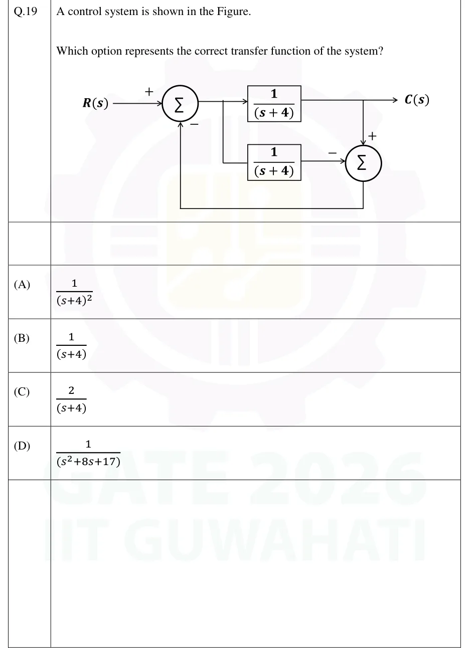
A control system is shown in the Figure.

Which option represents the correct transfer function of the system?

GATE 2026 EC question 19: Block diagram. — Figure from the GATE 2026 EC paper. It is part of the question.

(A)
$\frac{1}{( s + 4 ) ^{2}}$
(B)
$\frac{1}{( s + 4 )}$
(C)
$\frac{2}{( s + 4 )}$
(D)
$\frac{1}{( s ^{2} + 8 s + 17 )}$

Answer and solution

GATE 2026 EC Q.19: answer and solution

GATE 2025 EC Q.56

GATE 2025 · ECQ.56 · 2 marks · MSQ

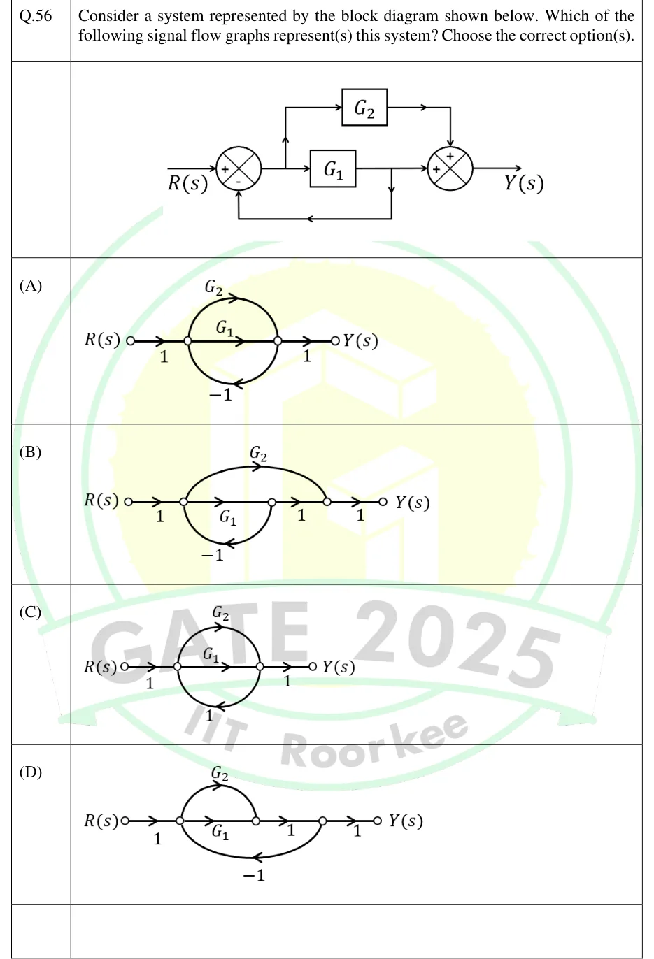
Consider a system represented by the block diagram shown below. Which of the following signal flow graphs represent(s) this system? Choose the correct option(s).

GATE 2025 EC question 56: Block diagram: R(s) enters the + input of summing junction 1. — Figure from the GATE 2025 EC paper. It is part of the question.

(A)
Figure: $R (s) 1 n_{1}$ ; $n_{1} G_{1} n_{2}$ (straight branch); $n_{1} G_{2} n_{2}$ (upper arc); $n_{2} - 1 n_{1}$ (lower arc, feedback); $n_{2} 1 Y (s)$ .
(B)
Figure: $R (s) 1 n_{1}$ ; $n_{1} G_{1} n_{2}$ ; $n_{2} 1 n_{3}$ ; $n_{1} G_{2} n_{3}$ (upper arc that skips $n_{2}$ ); $n_{2} - 1 n_{1}$ (lower arc, feedback); $n_{3} 1 Y (s)$ .
(C)
Figure: $R (s) 1 n_{1}$ ; $n_{1} G_{1} n_{2}$ (straight branch); $n_{1} G_{2} n_{2}$ (upper arc); $n_{2} 1 n_{1}$ (lower arc, feedback gain $+ 1$ ); $n_{2} 1 Y (s)$ .
(D)
Figure: $R (s) 1 n_{1}$ ; $n_{1} G_{1} n_{2}$ (straight branch); $n_{1} G_{2} n_{2}$ (upper arc); $n_{2} 1 n_{3}$ ; $n_{3} - 1 n_{1}$ (lower arc from $n_{3}$ back to $n_{1}$ , feedback); $n_{3} 1 Y (s)$ .

Answer and solution

GATE 2025 EC Q.56: answer and solution

GATE 2024 EE Q.20

GATE 2024 · EEQ.20 · 1 mark · MCQ

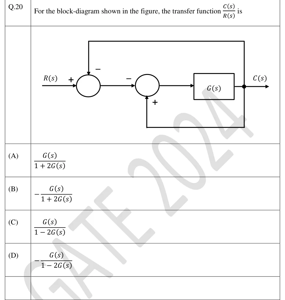
For the block-diagram shown in the figure, the transfer function $\frac{C ( s )}{R ( s )}$ is

GATE 2024 EE question 20: Two summing junctions in cascade followed by a single forward block G(s). — Figure from the GATE 2024 EE paper. It is part of the question.

(A)
$\frac{G ( s )}{1 + 2 G ( s )}$
(B)
$- \frac{G ( s )}{1 + 2 G ( s )}$
(C)
$\frac{G ( s )}{1 - 2 G ( s )}$
(D)
$- \frac{G ( s )}{1 - 2 G ( s )}$

Answer and solution

GATE 2024 EE Q.20: answer and solution

GATE 2023 EC Q.42

GATE 2023 · ECQ.42 · 2 marks · MCQ

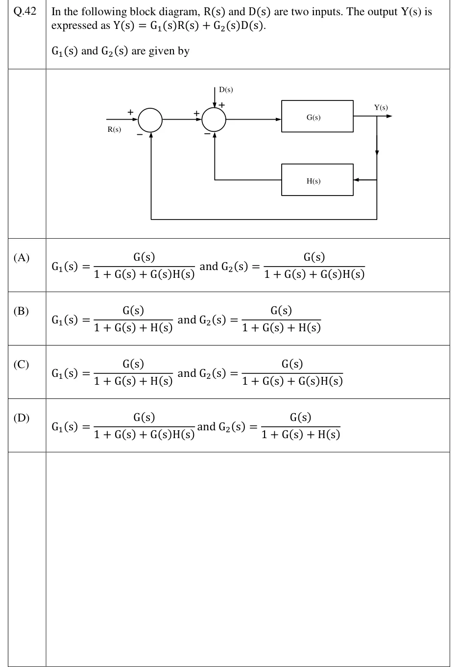
In the following block diagram, $R (s)$ and $D (s)$ are two inputs. The output $Y (s)$ is expressed as $Y (s) = G_{1} (s) R (s) + G_{2} (s) D (s)$ .

$G_{1} (s)$ and $G_{2} (s)$ are given by

GATE 2023 EC question 42: Two summing junctions in cascade, then a forward block G(s) whose output is Y(s). — Figure from the GATE 2023 EC paper. It is part of the question.

(A)
$G_{1} (s) = \frac{G ( s )}{1 + G ( s ) + G ( s ) H ( s )}$ and $G_{2} (s) = \frac{G ( s )}{1 + G ( s ) + G ( s ) H ( s )}$
(B)
$G_{1} (s) = \frac{G ( s )}{1 + G ( s ) + H ( s )}$ and $G_{2} (s) = \frac{G ( s )}{1 + G ( s ) + H ( s )}$
(C)
$G_{1} (s) = \frac{G ( s )}{1 + G ( s ) + H ( s )}$ and $G_{2} (s) = \frac{G ( s )}{1 + G ( s ) + G ( s ) H ( s )}$
(D)
$G_{1} (s) = \frac{G ( s )}{1 + G ( s ) + G ( s ) H ( s )}$ and $G_{2} (s) = \frac{G ( s )}{1 + G ( s ) + H ( s )}$

Answer and solution

GATE 2023 EC Q.42: answer and solution

GATE 2023 EE Q.12

GATE 2023 · EEQ.12 · 1 mark · MCQ

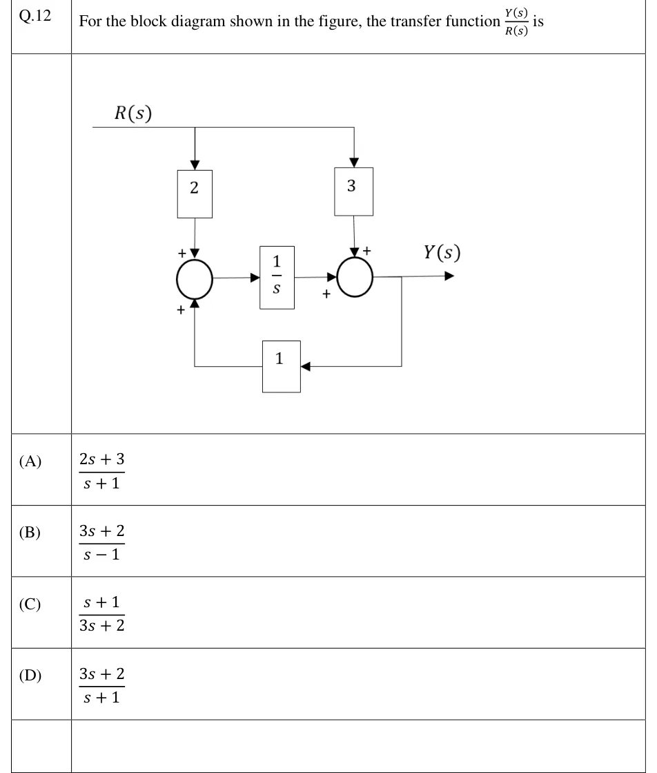
For the block diagram shown in the figure, the transfer function $\frac{Y ( s )}{R ( s )}$ is

GATE 2023 EE question 12: Input R(s) enters from the left on a horizontal line that branches to two blocks. — Figure from the GATE 2023 EE paper. It is part of the question.

(A)
$\frac{2 s + 3}{s + 1}$
(B)
$\frac{3 s + 2}{s - 1}$
(C)
$\frac{s + 1}{3 s + 2}$
(D)
$\frac{3 s + 2}{s + 1}$

Answer and solution

GATE 2023 EE Q.12: answer and solution

GATE 2022 IN Q.11

GATE 2022 · INQ.11 · 1 mark · MCQ

The input $x (t)$ to a system is related to its output $y (t)$ as

\frac{d y ( t )}{d t} + y (t) = 3 x (t - 3) u (t - 3)

Here $u (t)$ represents a unit-step function. The transfer function of this system is ________

(A)
$\frac{e ^{- 3 s}}{s + 3}$
(B)
$\frac{3 e ^{- 3 s}}{s + 1}$
(C)
$\frac{3 e ^{- (s /3)}}{s + 1}$
(D)
$\frac{e ^{- (s /3)}}{s + 3}$

Answer and solution

GATE 2022 IN Q.11: answer and solution

See the question in the paper

Tap to open full size

GATE 2022 IN Q.11: answer and solution

GATE 2022 IN Q.37

GATE 2022 · INQ.37 · 2 marks · MCQ

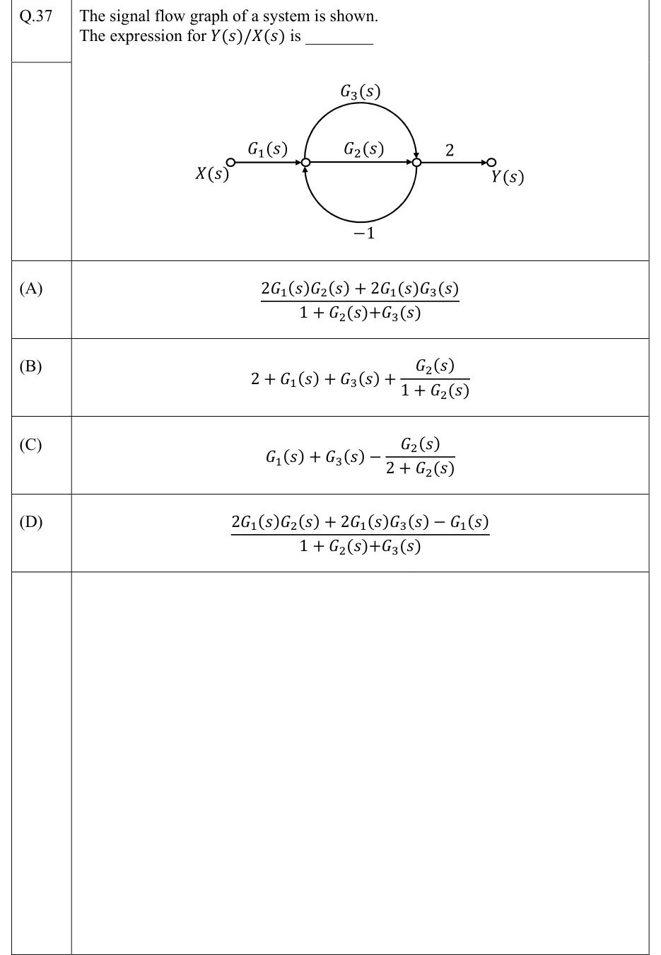
The signal flow graph of a system is shown. The expression for $Y (s) / X (s)$ is ________

GATE 2022 IN question 37: Signal flow graph with four nodes in a row: input node X(s), node A, node B and output node Y(s). — Figure from the GATE 2022 IN paper. It is part of the question.

(A)
$\frac{2 G _{1} ( s ) G _{2} ( s ) + 2 G _{1} ( s ) G _{3} ( s )}{1 + G _{2} ( s ) + G _{3} ( s )}$
(B)
$2 + G_{1} (s) + G_{3} (s) + \frac{G _{2} ( s )}{1 + G _{2} ( s )}$
(C)
$G_{1} (s) + G_{3} (s) - \frac{G _{2} ( s )}{2 + G _{2} ( s )}$
(D)
$\frac{2 G _{1} ( s ) G _{2} ( s ) + 2 G _{1} ( s ) G _{3} ( s ) - G _{1} ( s )}{1 + G _{2} ( s ) + G _{3} ( s )}$

Answer and solution

GATE 2022 IN Q.37: answer and solution

GATE 2020 EE Q.10

GATE 2020 · EEQ.10 · 1 mark · MCQ

Consider a linear time-invariant system whose input $r (t)$ and output $y (t)$ are related by the following differential equation:

\frac{d ^{2} y ( t )}{d t ^{2}} + 4 y (t) = 6 r (t)

The poles of this system are at

(A)
$+ 2 j, - 2 j$
(B)
$+ 2, - 2$
(C)
$+ 4, - 4$
(D)
$+ 4 j, - 4 j$

Answer and solution

GATE 2020 EE Q.10: answer and solution

See the question in the paper

Tap to open full size

GATE 2020 EE Q.10: answer and solution

GATE 2020 EE Q.13

GATE 2020 · EEQ.13 · 1 mark · MCQ

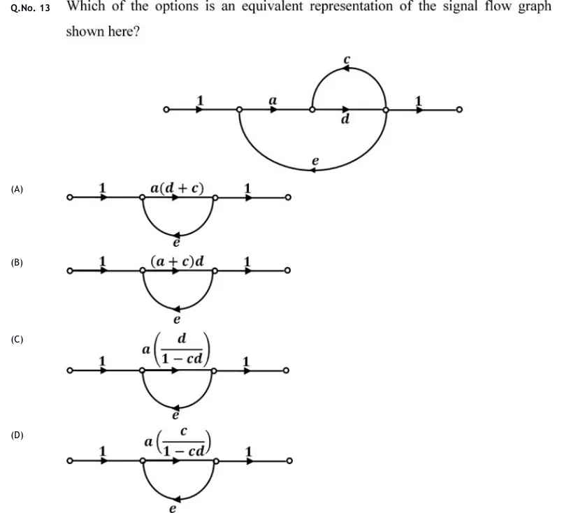
Which of the options is an equivalent representation of the signal flow graph shown here?

GATE 2020 EE question 13: Signal flow graph with five nodes on a horizontal line: input node x_0, then x_1, x_2, x_3, output node x_4. — Figure from the GATE 2020 EE paper. It is part of the question.

(A)
Figure — input $1$ P $a (d + c)$ Q $1$ output, feedback branch $e$ from Q to P
(B)
Figure — input $1$ P $(a + c) d$ Q $1$ output, feedback branch $e$ from Q to P
(C)
Figure — input $1$ P $a (\frac{d}{1 - c d})$ Q $1$ output, feedback branch $e$ from Q to P
(D)
Figure — input $1$ P $a (\frac{c}{1 - c d})$ Q $1$ output, feedback branch $e$ from Q to P

Answer and solution

GATE 2020 EE Q.13: answer and solution

GATE 2018 EC Q.4

GATE 2018 · ECQ.4 · 1 mark · MCQ

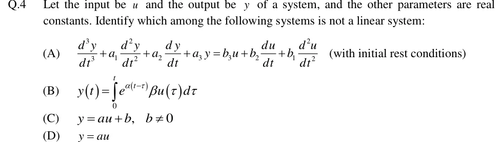
Let the input be $u$ and the output be $y$ of a system, and the other parameters are real constants. Identify which among the following systems is not a linear system:

(A)
$\frac{d ^{3} y}{d t ^{3}} + a_{1} \frac{d ^{2} y}{d t ^{2}} + a_{2} \frac{d y}{d t} + a_{3} y = b_{3} u + b_{2} \frac{d u}{d t} + b_{1} \frac{d ^{2} u}{d t ^{2}}$ (with initial rest conditions)
(B)
$y (t) = \int_{0}^{t} e^{α (t - τ)} β u (τ) d τ$
(C)
$y = a u + b, b \neq = 0$
(D)
$y = a u$

Answer and solution

GATE 2018 EC Q.4: answer and solution

See the question in the paper

Tap to open full size

GATE 2018 EC Q.4: answer and solution

PRACTICE

7 questions to test yourself

PRACTICE 11 mark · NAT

A plant $G (s) = \frac{K}{s + 2}$ with nominal $K = 18$ is placed in a unity negative-feedback loop. The sensitivity of the closed-loop DC gain $T (0)$ to $K$ , $S_{K}^{T} = \frac{\partial T / T}{\partial K / K}$ , evaluated at the nominal value, is ______ (to two decimal places).

Answer and solution

Answer: $0.1$ (accepted range $\pm 0.005$ )

$T (s) = \frac{K}{s + 2 + K}$ , so the DC gain is $T (0) = \frac{K}{K + 2}$ .
$\frac{\partial T ( 0 )}{\partial K} = \frac{2}{( K + 2 ) ^{2}}$ , so $S_{K}^{T} = \frac{K}{T ( 0 )} \cdot \frac{2}{( K + 2 ) ^{2}} = \frac{2}{K + 2}$ .
At $K = 18$ : $S_{K}^{T} = 2/20 = 0.10$ . Check: $1/ (1 + G (0)) = 1/ (1 + 9) = 0.10$ .

PRACTICE 22 marks · MCQ

A signal flow graph has nodes $x_{1}$ (input) to $x_{5}$ and exactly these branches: $x_{1} \to x_{2}$ : $1$ ; $x_{2} \to x_{3}$ : $a$ ; $x_{3} \to x_{4}$ : $b$ ; $x_{4} \to x_{5}$ : $c$ ; $x_{3} \to x_{2}$ : $- d$ ; $x_{4} \to x_{3}$ : $- e$ ; $x_{5} \to x_{4}$ : $- f$ ; $x_{1} \to x_{4}$ : $g$ . The transfer function $x_{5} / x_{1}$ is

(A)
$\frac{ab c + c g}{1 + a d + b e + c f + a c df}$
(B)
$\frac{ab c + c g ( 1 + a d )}{1 + a d + b e + c f + a c df}$
(C)
$\frac{ab c + c g ( 1 + a d )}{1 + a d + b e + c f}$
(D)
$\frac{ab c + c g ( 1 + b e )}{1 + a d + b e + c f + a c df}$

Answer and solution

Answer: (B)

Loops: $L_{1} = a (- d) = - a d$ on $x_{2}, x_{3}$ ; $L_{2} = b (- e) = - b e$ on $x_{3}, x_{4}$ ; $L_{3} = c (- f) = - c f$ on $x_{4}, x_{5}$ . Every feedback branch spans only one step, so any longer closed path would have to revisit a node. There are no other loops.
Non-touching pairs: only $L_{1}$ and $L_{3}$ (nodes ${x_{2}, x_{3}}$ and ${x_{4}, x_{5}}$ ). $L_{1}$ and $L_{2}$ share $x_{3}$ ; $L_{2}$ and $L_{3}$ share $x_{4}$ .
$Δ = 1 - (L_{1} + L_{2} + L_{3}) + L_{1} L_{3} = 1 + a d + b e + c f + a c df$ .
Forward paths: $P_{1} = ab c$ passes through every node and touches all loops, so $Δ_{1} = 1$ . $P_{2} = g c$ runs $x_{1} \to x_{4} \to x_{5}$ and does not touch $L_{1}$ , so $Δ_{2} = 1 - L_{1} = 1 + a d$ .
$\frac{x _{5}}{x _{1}} = \frac{ab c + c g ( 1 + a d )}{1 + a d + b e + c f + a c df}$ . Check with every gain equal to 1: Mason gives $3/5$ , and solving the node equations directly also gives $x_{5} = 0.6 x_{1}$ .

PRACTICE 32 marks · MSQ

A plant $G (s) = \frac{K}{τ s + 1}$ with $K > 0$ and $τ > 0$ is in a unity negative-feedback loop. A disturbance $d (t)$ is added directly to the plant output. Sensor noise $n (t)$ is added to the measured output, so the comparator forms $e = r - (y + n)$ . Which of the following statements are correct?

(A)
The closed-loop DC gain from $r$ to $y$ is $\frac{K}{1 + K}$ .
(B)
The closed-loop $- 3$ dB bandwidth from $r$ to $y$ is $\frac{1 + K}{τ}$ rad/s.
(C)
As $K \to \infty$ , the steady-state output caused by a constant sensor noise $n$ tends to zero.
(D)
For a unit-step disturbance $d (t)$ with $r = n = 0$ , the steady-state output is $\frac{1}{1 + K}$ .

Answer and solution

Answer: (A), (B), (D)

$Y = G (R - Y - N) + D$ , so $Y = \frac{G}{1 + G} (R - N) + \frac{1}{1 + G} D$ .
A: $\frac{G ( 0 )}{1 + G ( 0 )} = \frac{K}{1 + K}$ . Correct.
B: $\frac{G}{1 + G} = \frac{K}{τ s + 1 + K}$ has a single pole at $s = - (1 + K) / τ$ , so the bandwidth is $(1 + K) / τ$ rad/s. Correct.
C: $Y / N = - \frac{G}{1 + G}$ , whose DC value $- \frac{K}{1 + K}$ tends to $- 1$ as $K \to \infty$ . The noise reaches the output almost in full, and raising the gain makes it worse. Incorrect.
D: $Y / D = \frac{1}{1 + G} = \frac{τ s + 1}{τ s + 1 + K}$ . The loop is stable, so by the final value theorem the unit-step response settles at $\frac{1}{1 + K}$ . Correct.

PRACTICE 42 marks · NAT

An armature-controlled DC motor has armature resistance $R_{a} = 2 Ω$ , negligible armature inductance, torque constant $K_{t} = 0.5$ N·m/A and back-emf constant $K_{b} = 0.5$ V·s/rad. The total inertia is $J = 0.02$ kg·m² and the viscous friction is $B = 0.05$ N·m·s/rad, both referred to the motor shaft. There is no load torque. A constant 12 V is applied to the armature with the motor starting from rest. The steady-state speed, in rad/s, is ______ (to two decimal places).

Answer and solution

Answer: $17.14$ (accepted range $\pm 0.05$ )

With $L_{a} = 0$ : $\frac{Ω ( s )}{V _{a} ( s )} = \frac{K _{t}}{R _{a} ( J s + B ) + K _{t} K _{b}}$ .
DC gain $= \frac{K _{t}}{R _{a} B + K _{t} K _{b}} = \frac{0.5}{2 ( 0.05 ) + 0.5 ( 0.5 )} = \frac{0.5}{0.35} = 1.4286$ (rad/s)/V.
Steady-state speed $= 12 \times 1.4286 = 17.14$ rad/s.
Physical check: armature current $= (12 - 0.5 \times 17.14) /2 = 1.714$ A, so the motor torque is $0.5 \times 1.714 = 0.857$ N·m. This equals the friction torque $B ω = 0.05 \times 17.14 = 0.857$ N·m.
$J$ sets only the time constant, $R_{a} J / (R_{a} B + K_{t} K_{b}) = 0.04/0.35 \approx 0.114$ s, and does not affect the final speed.

PRACTICE 52 marks · MCQ

In a block diagram, the reference $R$ enters a first summing point. Its other input is the output $C$ fed back through $H$ with a minus sign. The output of the first summing point drives $G_{1}$ . At a second summing point, the output of $G_{1}$ is added to a feedforward signal $G_{3} R$ taken directly from $R$ . The output of the second summing point drives $G_{2}$ , whose output is $C$ . The transfer function $C (s) / R (s)$ is

(A)
$\frac{G _{1} G _{2} + G _{3}}{1 + G _{1} G _{2} H}$
(B)
$\frac{G _{2} ( G _{1} + G _{3} )}{1 + G _{1} G _{2} H + G _{2} G _{3} H}$
(C)
$\frac{G _{2} ( G _{1} + G _{3} )}{1 + G _{1} G _{2} H}$
(D)
$\frac{G _{1} G _{2} ( 1 + G _{3} )}{1 + G _{1} G _{2} H}$

Answer and solution

Answer: (C)

Call the output of the first summing point $E$ . Then $E = R - H C$ and $C = G_{2} (G_{1} E + G_{3} R)$ .
Substitute: $C = G_{1} G_{2} R - G_{1} G_{2} H C + G_{2} G_{3} R$ , so $C (1 + G_{1} G_{2} H) = G_{2} (G_{1} + G_{3}) R$ .
$\frac{C}{R} = \frac{G _{2} ( G _{1} + G _{3} )}{1 + G _{1} G _{2} H}$ .
Mason check: the forward paths are $P_{1} = G_{1} G_{2}$ and $P_{2} = G_{3} G_{2}$ . The only loop is $L_{1} = - G_{1} G_{2} H$ . The feedforward branch starts at the source node $R$ , so it forms no loop, which rules out option B. Both forward paths pass through the second summing node and $C$ , which lie on the loop, so $Δ_{1} = Δ_{2} = 1$ .
Option A forgets that the feedforward signal also passes through $G_{2}$ . Option D treats the feedforward as a multiplying factor instead of adding it at the summing point.

PRACTICE 61 mark · NAT

A motor drives a load through an ideal gear pair. The motor-side gear has 20 teeth and the load-side gear has 100 teeth. The motor rotor inertia is 0.01 kg·m² and the load inertia is 1 kg·m²; the gear inertias are negligible. The total inertia referred to the motor shaft, in kg·m², is ______ (to two decimal places).

Answer and solution

Answer: $0.05$ (accepted range $\pm 0.002$ )

Refer the load inertia to the motor shaft with the factor $(N_{1} / N_{2})^{2} = (20/100)^{2} = 0.04$ .
$J_{e q} = J_{m} + 0.04 J_{L} = 0.01 + 0.04 \times 1 = 0.05$ kg·m².
Energy check: the load turns at $ω_{L} = 0.2 ω_{m}$ , so the total kinetic energy is $\frac{1}{2} (0.01 + 1 \times 0. 2^{2}) ω_{m}^{2} = \frac{1}{2} (0.05) ω_{m}^{2}$ .

PRACTICE 71 mark · MCQ

In the force-current analogy, the stiffness $K$ of a translational spring is analogous to

(A)
Capacitance $C$
(B)
Inductance $L$
(C)
Reciprocal of inductance, $1/ L$
(D)
Reciprocal of capacitance, $1/ C$

Answer and solution

Answer: (C)

In the force-current analogy, force corresponds to current and velocity $u$ corresponds to voltage $v$ .
Spring: $f = K \int u d t$ . Inductor: $i = \frac{1}{L} \int v d t$ .
Matching term by term gives $K \leftrightarrow 1/ L$ . Option D, $1/ C$ , is the force-voltage answer, where $f = K \int u d t$ is matched with $v = \frac{1}{C} \int i d t$ .

OFFICIAL GATE 2027 SYLLABUS WORDING

Copied from the GATE 2027 syllabus; see all 2027 syllabi.

GATE EC

Basic control system components; Feedback principle; Transfer function; Block diagram representation; Signal flow graph

GATE EE

Mathematical modelling and representation of systems, Feedback principle, transfer function, Block diagrams and Signal flow graphs

GATE IN

Feedback principles, role of sensing in feedback, signal flow graphs

Preparing in Kolkata? IAE Academy's course for GATE ECE, GATE EE or GATE IN.