GATE 2025 IN Q.37
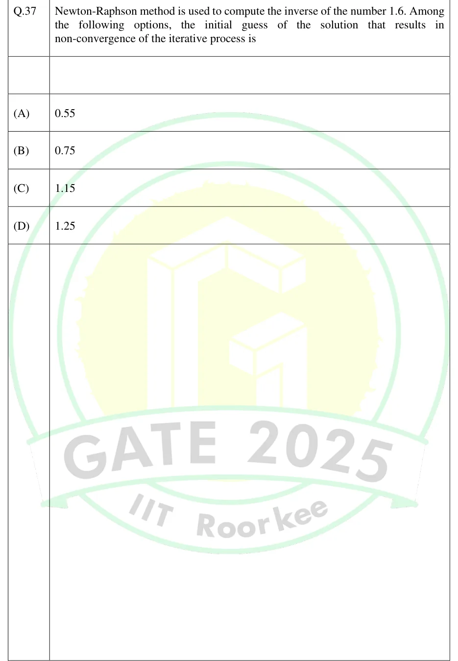
Newton-Raphson method is used to compute the inverse of the number 1.6. Among the following options, the initial guess of the solution that results in non-convergence of the iterative process is
- (A)
0.55
- (B)
0.75
- (C)
1.15
- (D)
1.25

IN THE IN SYLLABUS
Numerical methods replace an exact closed-form answer with a finite, repeatable calculation: an iteration that closes in on the solution of a linear system or on a root of , a weighted sum of function values that approximates an integral, a step-by-step march along the solution of a differential equation, and a least-squares fit to data. A hand calculation here usually means carrying out one or two steps of a named method, so what counts is knowing each formula exactly, the condition it needs (a sign change, an even number of intervals, diagonal dominance) and its order of accuracy or convergence. The IN syllabus also names backpropagation, which is the chain rule applied to a small network followed by one gradient-descent update.
6 previous-year questions · 6 solved · 6 practice questions
A system of equations in unknowns has a unique solution exactly when . Everything in these notes is real-valued. Direct methods (Gaussian elimination, LU decomposition) reach the solution in a fixed number of arithmetic operations, apart from rounding. Iterative methods (Gauss-Jacobi, Gauss-Seidel) start from a guess and improve it sweep by sweep; each sweep is cheap, but they converge only under conditions on .
Gaussian elimination, step by step:
Write the augmented matrix .
For each column , use row (the pivot row) to make every entry below zero: with multiplier , using the current (already reduced) entries.
With partial pivoting, first swap into row the row (from row downwards) whose entry in column has the largest absolute value. This avoids dividing by a zero or a very small pivot.
The result is an upper-triangular system . Solve it by back substitution: first, then , and so on up.
= product of the pivots, times for every row swap made.
Cost: elimination takes about multiplications and divisions, back substitution about .
LU DECOMPOSITION
Doolittle form: is unit lower triangular (1s on its diagonal) and holds the multipliers below the diagonal; is the upper-triangular matrix that Gaussian elimination without row swaps produces. Crout form puts the 1s on the diagonal of instead. For a non-singular , the factorisation exists without row swaps exactly when every leading principal minor of is non-zero. One factorisation serves any number of right-hand sides .
For example, : the multiplier goes into , and is the second pivot. A symmetric positive definite matrix can also be factorised as with lower triangular and positive on its diagonal (Cholesky).
GAUSS-JACOBI ITERATION
Every new component uses only the previous sweep's values. Needs (reorder the equations if necessary).
GAUSS-SEIDEL ITERATION
Each new component is used immediately, later in the same sweep. Needs .
ITERATION MATRICES AND THE CONVERGENCE TEST
Here is the diagonal of and , are its strictly lower and strictly upper triangular parts (not the LU factors). Each method has the form , and , the spectral radius, is the largest over the eigenvalues of .
STRICT DIAGONAL DOMINANCE (SUFFICIENT CONDITION)
If it holds, both Jacobi and Gauss-Seidel converge for every starting vector. It is sufficient, not necessary: a system that fails it may still converge. Gauss-Seidel also converges for every start when is symmetric positive definite.
WORKED EXAMPLE
Solve , , by Gauss-Seidel from . Give the first two iterates, and compare with one Jacobi sweep.
Check convergence first: , , . The system is strictly diagonally dominant, so Gauss-Seidel converges from any start.
Solve each equation for its diagonal unknown: , , .
Sweep 1: ; then, with the new , ; then .
Sweep 2: , , .
Jacobi uses only old values, so its first sweep is , , , further from the solution than the Gauss-Seidel iterate.
Substitution confirms that the exact solution is , which the Gauss-Seidel iterates are approaching.
Answer: Gauss-Seidel: , then . Jacobi's first sweep: . Exact: .
EXAM TIP
Gauss-Seidel usually needs fewer sweeps than Jacobi, but not always. For any system with non-zero diagonal entries (and more generally any tridiagonal one) : the two methods converge or diverge together, and asymptotically, when they converge, one Gauss-Seidel sweep reduces the error about as much as two Jacobi sweeps. If a given system is not diagonally dominant, try reordering the equations before concluding anything about convergence.
To solve , generate a sequence that approaches a root ; the error is . Bracketing methods (bisection, regula falsi) keep an interval on which changes sign and always converge for a continuous . Open methods (Newton-Raphson, secant, fixed-point iteration) are faster near the root but can fail. Evaluate trigonometric functions in radians.
ORDER OF CONVERGENCE P
is linear (it also needs ; the error shrinks by a roughly constant factor each step). is superlinear. is quadratic: the number of correct digits roughly doubles each step.
BISECTION
Needs continuous on with ; keep the half on which the sign still changes. The -th midpoint is within of a root, and the bracket after halvings has that length. The error bound halves at every step, which is why bisection is counted as linearly convergent with ratio ; the actual error need not decrease at every step. The number of steps for a tolerance does not depend on .
REGULA FALSI (FALSE POSITION)
The -intercept of the chord joining and . Needs , and the new bracket is whichever of , keeps the sign change. Always converges for continuous , but usually only linearly, because one end of the bracket often stays fixed.
NEWTON-RAPHSON
The -intercept of the tangent at . For continuous near a simple root (), convergence from a start close enough to the root is at least quadratic (faster when ). At a root of multiplicity it is only linear, with ; the modified step restores quadratic convergence.
NEWTON-RAPHSON FOR ROOTS AND RECIPROCALS
From , and respectively, with . The iteration converges from every (after the first step every iterate is at least , and they decrease). The reciprocal iteration uses no division; since , it converges to exactly when .
SECANT
Newton-Raphson with replaced by the slope through the last two iterates. Needs two starting values but no derivative and no sign change. Order near a simple root; it can diverge because it does not keep a bracket.
FIXED-POINT ITERATION
Rewrite as , with continuous near . Linear convergence with ratio when ; the iterates move away if . Interval test: if maps into itself and for all in , then contains exactly one fixed point and the iteration converges to it from every in . Newton-Raphson is the choice , for which at a simple root, which is why it is faster than linear.
Method | Starting data | Keeps a bracket? | Order near a simple root | Can it fail? |
|---|---|---|---|---|
Bisection | with | Yes | 1 (error bound halves each step) | No, for continuous |
Regula falsi | with | Yes | 1 | No, for continuous (but can be slow) |
Secant | No | Yes, it can diverge | ||
Newton-Raphson | and | No | 2 | Yes: , cycling, divergence |
Fixed point | and | No | 1 when | Yes, when |
When Newton-Raphson goes wrong:
(horizontal tangent): the step is undefined, and a nearly zero throws the next iterate far away.
Cycling: for from the iterates are for ever.
Divergence: for the step gives , so from any the iterates run away from the root at .
A start far from the wanted root can converge to a different root.
At a multiple root the method still converges from nearby, but only linearly.
WORKED EXAMPLE
Find the real root of by Newton-Raphson from , correct to four decimal places.
, for all , so is increasing and has exactly one real root; and place it in .
.
and , so .
and , so . The next step changes by only about (to ), so the first four decimal places are settled.
Errors: , , . The ratios and approach : quadratic convergence. (The first step, taken far from the root, does not follow this ratio yet.)
Answer:
EXAM TIP
Choosing matters. For (root ): has and diverges (from : ); has , so iterates near also move away from it; has and converges (from : ), overshooting alternately because .
EXAM TIP
Bisection counting: on with tolerance , , so steps. Conventions differ by one, because the bracket after halvings has length while the midpoint of that bracket is within of the root. Read which quantity the question bounds.
EXAM TIP
Regula falsi and the secant method use the same chord formula. Regula falsi keeps whichever old point preserves the sign change; the secant method always discards the older point. Same formula, different bookkeeping, different guarantees.
Divide into equal subintervals of width , with nodes and ordinates for , which makes points. Each rule replaces on a panel by the polynomial through its points and integrates that polynomial exactly. Error convention used below: , with some point in .
COMPOSITE TRAPEZOIDAL RULE
Any . A straight line on each subinterval. Exact for polynomials of degree .
TRAPEZOIDAL ERROR
Global error : halving cuts the error by a factor of about 4. If on (convex ) the rule overestimates; if it underestimates.
COMPOSITE SIMPSON'S 1/3 RULE
must be even (an odd number of points). A parabola through each pair of subintervals. Exact for polynomials of degree .
SIMPSON'S 1/3 ERROR
Global error : halving cuts the error by a factor of about 16.
COMPOSITE SIMPSON'S 3/8 RULE
must be a multiple of 3. A cubic through each group of three subintervals. Exact for polynomials of degree , the same degree as the 1/3 rule.
SIMPSON'S 3/8 ERROR
Also globally, with a larger constant than the 1/3 rule at the same . Useful when is odd and at least 3: apply the 3/8 rule to three subintervals and the 1/3 rule to the rest.
Rule | Allowed n | Weights (multiply by ) | Exact up to degree | Error on one panel | Global error |
|---|---|---|---|---|---|
Trapezoidal | any | 1 | |||
Simpson's 1/3 | even | 3 | |||
Simpson's 3/8 | multiple of 3 | 3 |
TWO-POINT GAUSS-LEGENDRE QUADRATURE
The second form follows from the substitution . Two function values at unequally placed points, yet exact for polynomials of degree , like Simpson's rules with three. Check: for it gives with , the exact value.
WORKED EXAMPLE
Estimate with subintervals by the trapezoidal rule and by Simpson's 1/3 rule, and check Simpson's error against its error formula.
. Ordinates at : .
Trapezoidal: .
Simpson's 1/3 ( is even): .
Exact value: . Trapezoidal error , an overestimate as expected because . Simpson error .
Simpson's error formula with (a constant, so does not matter): , exactly the observed error.
Answer: Trapezoidal , Simpson's 1/3 , exact .
EXAM TIP
Count intervals, not points: subintervals means ordinates. Simpson's 1/3 rule needs an odd number of ordinates (); the 3/8 rule needs . Because both Simpson rules are exact for cubics, the error of either one on a polynomial of degree is exactly .
EXAM TIP
If a table gives values at unequal spacing, none of these formulas applies as written. Apply the trapezoidal rule interval by interval, each with its own width.
For the initial-value problem , , a one-step method advances from to . A method of order has local truncation error (the error made in one step, starting from exact data) and global error (accumulated at a fixed after about steps) . Halving divides the global error by about .
EULER (EXPLICIT, FORWARD)
Follows the tangent line at the start of the step. Order 1: local error , global error .
BACKWARD (IMPLICIT) EULER
Order 1, but appears on both sides and must be solved for (directly when is linear in ). For with real it gives , which decays for every .
MODIFIED EULER (HEUN), A SECOND-ORDER RUNGE-KUTTA METHOD
An Euler predictor followed by a trapezoidal corrector. Order 2: local error , global error . The same computation written as , , is one second-order Runge-Kutta method; the midpoint method below is another. Some texts apply the corrector repeatedly, putting each new back into until two successive values agree; one application is the formula above.
RUNGE-KUTTA, FOURTH ORDER (CLASSICAL)
Four evaluations of per step. Order 4: local error , global error . Note that uses , not , and uses a full step with .
TAYLOR-SERIES METHOD
The higher derivatives come from differentiating the equation itself (, are partial derivatives, evaluated at ). Truncating after the term gives a method of order ; keeping only the term is Euler's method.
PICARD'S SUCCESSIVE APPROXIMATIONS
Each iterate is a function, not a number. For , : , , and each further iterate adds the next term of the series of .
STABILITY OF EXPLICIT EULER
real. For the numerical solution decays without changing sign, like the exact ; at it is after one step. For it alternates in sign while decaying. At it alternates with constant magnitude, and for it grows without bound.
Method | Evaluations of f per step | Local error | Global error (order) |
|---|---|---|---|
Euler (forward or backward) | 1 | (1) | |
Modified Euler (Heun) / RK2 | 2 | (2) | |
Runge-Kutta 4 | 4 | (4) |
WORKED EXAMPLE
For , , take one step of with Euler, modified Euler (Heun) and RK4, and compare with the exact .
Euler: .
Heun: predictor ; ; corrector .
RK4: ; ; ; .
.
Exact solution: (check: and ), so . Errors: Euler , Heun , RK4 .
Answer: (Euler), (Heun), (RK4); exact .
EXAM TIP
Naming convention: in these notes, modified Euler means Heun's predictor-corrector above. Some texts give that name to the midpoint method, , which is also second order but gives different numbers. If a question writes out its formula, use that formula.
EXAM TIP
When depends on only, is just an integral: Heun's method becomes the trapezoidal rule over the step, and RK4 becomes Simpson's 1/3 rule on with half-width . This gives a quick check on an RK4 calculation.
EXAM TIP
A second-order equation becomes the first-order system , with and given. Apply the method to both components together; with Euler, and , both from the old values.
EXAM TIP
Keep local and global error apart. Euler's local error is but its global error is ; a method described as order has global error .
Given data , , the least-squares line chooses and to minimise the sum of squared vertical deviations . Setting and gives the normal equations. Notation: , , , , . Where , appear below, any one divisor ( or ) may be used for the variances and the covariance, as long as it is the same for all of them: every formula here is a ratio in which it cancels.
NORMAL EQUATIONS FOR Y = A + BX
Two linear equations in and . For a parabola the same method gives three: , , . For a line through the origin, , the single normal equation gives .
LEAST-SQUARES SLOPE AND INTERCEPT (REGRESSION OF Y ON X)
The line passes through and its residuals sum to zero. It minimises vertical deviations, so it is the line for predicting from .
CORRELATION COEFFICIENT (PEARSON)
Defined only when neither nor is zero. , and exactly when all the points lie on one (non-horizontal, non-vertical) line. is unchanged by a change of origin and scale, , with ; if only its sign changes. It measures linear association only: for and , so , although is a function of .
THE TWO REGRESSION LINES
Both lines pass through , so when solving them together gives the means. The two coefficients have the sign of , and with that common sign. The lines coincide only when ; when they are and , perpendicular. The coefficients are unchanged by a change of origin but not of scale: with , , .
COEFFICIENT OF DETERMINATION
For the least-squares line (with an intercept), is the fraction of the variation of about that the line accounts for.
SPEARMAN'S RANK CORRELATION
Rank the values and the values separately; is the difference between the two ranks of item . This form is exact when there are no tied ranks (it is then Pearson's computed on the ranks). .
WORKED EXAMPLE
Fit by least squares to , find the correlation coefficient, and predict at .
, , .
Deviations: and .
, , .
and , so .
, and : the line accounts for about 96% of the variation in .
Prediction: . This is an extrapolation beyond the data, so treat it with caution.
Answer: , , .
EXAM TIP
Given two regression lines, say and : solving them together gives the means, , . To decide which line is on , try one assignment. Taking the first as on gives and the second as on gives ; the product is allowed, so . The other assignment gives , and a product of , which is impossible.
EXAM TIP
Linearise before fitting: for fit a straight line to ; for fit one to . The result minimises the squared error in , not in .
Training a neural network means adjusting its weights to reduce a loss . Gradient descent moves every weight a small step against its partial derivative. Backpropagation is the way those partial derivatives are computed: the chain rule applied from the output back towards the input, so that each layer reuses the derivative already found for the layer after it. The level needed here is a forward pass through a small network, the chain rule, and one update.
GRADIENT-DESCENT UPDATE
is the learning rate. Every partial derivative is evaluated at the current (old) weights, and then all the weights are updated together.
SQUARED-ERROR LOSS
is the network output and the target. The factor is a convention that cancels the 2 from differentiation; without it every gradient doubles, so check which form a question uses.
CHAIN RULE FOR ONE NEURON
is the neuron's input (the previous layer's output) and its activation. The last result is what is passed backwards to the previous layer.
BACKPROPAGATION THROUGH A LAYER
is the weight from unit into unit , and the sum runs over every unit that unit feeds. A unit feeding several others collects a contribution from each. For an output unit with the squared-error loss above, .
ACTIVATION FUNCTIONS AND THEIR DERIVATIVES
is largest, , at . The ReLU derivative is undefined at itself; a question that lands there should state the value it uses.
SIGMOID OUTPUT WITH CROSS-ENTROPY LOSS
is 0 or 1 (natural logarithm). The chain rule gives , and multiplying by cancels the denominator.
Backpropagation for input , one sigmoid hidden unit and a linear output:
Forward pass: , , , then . Keep , and .
Output: (linear output unit, squared-error loss with the ).
Output-layer gradients: and .
Propagate back: , using the old .
Hidden-layer gradients: and .
Update every parameter with .
WORKED EXAMPLE
In the network above, take , , , , , and learning rate . Carry out one gradient-descent update of all four parameters.
Forward: , , , .
Output: , so and .
Back to the hidden unit: , so .
Hidden gradients: and .
Update: , , , .
Check: a new forward pass gives , , and , down from .
Answer: , , , .
EXAM TIP
Use the old weights throughout the backward pass: needs as it was before its update. Updating first and then using the new value in is a different, incorrect computation.
PREVIOUS-YEAR QUESTIONS
Try each question first, then open the answer. We placed each question under a topic ourselves; the exam paper does not label topics.
See these papers in full: GATE EE 2023 · GATE EE 2018 · GATE IN 2025 · GATE IN 2024 · GATE IN 2022 · GATE IN 2020
Newton-Raphson method is used to compute the inverse of the number 1.6. Among the following options, the initial guess of the solution that results in non-convergence of the iterative process is
0.55
0.75
1.15
1.25
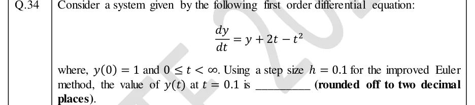
Consider a system given by the following first order differential equation:
where, and . Using a step size for the improved Euler method, the value of at is ________ (rounded off to two decimal places).
In the following differential equation, the numerically obtained value of , at , is ________ (Round off to 2 decimal places).
The Newton-Raphson method is applied to determine the solution of where . If the initial guess of the solution is , the value of the next approximation is ________ (round off to two decimal places)
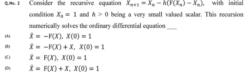
Consider the recursive equation , with initial condition and being a very small valued scalar. This recursion numerically solves the ordinary differential equation ____
The per-unit power output of a salient-pole generator which is connected to an infinite bus, is given by the expression, , where is the load angle. Newton-Raphson method is used to calculate the value of for pu. If the initial guess is , then its value (in degree) at the end of the first iteration is
PRACTICE
The system , is solved by the Gauss-Seidel method, updating first and then in each iteration, starting from , . The value of after the first iteration is ______ (rounded off to two decimal places).
Answer: (accepted range )
The system is strictly diagonally dominant (, ), so the iteration converges.
.
Gauss-Seidel uses the new at once: .
For comparison, Jacobi would give ; the exact solution is , .
The Newton-Raphson method is applied to with a starting value close to, but not equal to, . The iterates converge to
quadratically, with
linearly, with
linearly, with
not at all, because at every iterate
Answer: (B)
is a root of multiplicity , so and the quadratic-convergence result, which needs , does not apply.
Let . Then and , so .
As , , which is for .
is non-zero at every iterate near (but not at) , so the method does not break down: the convergence is linear with ratio . Answer (B).
For with , the approximate value of obtained by the classical fourth-order Runge-Kutta method with a single step is ______ (rounded off to four decimal places).
Answer: (accepted range )
, , , .
.
.
.
.
.
Check: the exact solution gives .
A network computes and , with loss . For input , target , initial weights , and learning rate , the value of after one gradient-descent update (all gradients evaluated at the initial weights) is ______ (rounded off to three decimal places).
Answer: (accepted range )
Forward: , so and ; .
.
Chain rule: .
Update: .
Which of the following statements is/are correct? Here is the number of equal subintervals and their width.
Simpson's 1/3 rule with gives the exact value of .
For an integrand whose fourth derivative is continuous and non-zero on the interval, halving in the composite Simpson's 1/3 rule reduces the error by a factor of about 4.
Simpson's 3/8 rule can be applied directly with .
The composite trapezoidal rule, for every , overestimates .
Answer: (A), (D)
(A) Correct. Simpson's rules are exact for polynomials of degree . Check: , at , so , and the exact value is .
(B) Incorrect. The composite Simpson error is , so halving reduces it by a factor of about .
(C) Incorrect. The 3/8 rule needs to be a multiple of 3, and 8 is not.
(D) Correct. , so is convex and every chord lies above the curve; equivalently , i.e. approximation > exact.
The two lines of regression of a bivariate data set are and . The correlation coefficient between and is ______ (rounded off to one decimal place).
Answer: (accepted range )
Both lines pass through the means. Solving them together: from the second, ; substituting, , so , and .
Try the first line as on : , so . The second as on : , so . The product is allowed.
The other assignment gives (from ) and (from ), a product of , which is impossible.
, and has the sign of the (positive) regression coefficients, so .
OFFICIAL GATE 2027 SYLLABUS WORDING
Copied from the GATE 2027 syllabus; see all 2027 syllabi.
GATE IN
Numerical Methods: Solution of matrix equations, solutions of non-linear algebraic equations, iterative methods for solving differential equations, numerical integration, regression and correlation analysis, backpropagation for neural networks
Preparing in Kolkata? IAE Academy's course for GATE IN.