GATE CS · DA

Greedy, dynamic programming and divide-and-conquer

Greedy, dynamic programming and divide-and-conquer are the three core algorithm-design paradigms for GATE CS. Greedy makes an irrevocable, locally best choice at each step, and it is correct only when this can be proved, usually with an exchange argument. Divide-and-conquer splits a problem into independent subproblems, solves them recursively and combines the results. Dynamic programming solves overlapping subproblems once each and reuses the stored answers. These notes cover the standard algorithms: activity selection, fractional knapsack, Huffman coding, job sequencing, merge sort, quicksort, binary search, maximum subarray (D&C and Kadane), counting inversions, Strassen, simultaneous max–min, LCS, edit distance, 0/1 knapsack, subset sum and matrix chain multiplication. They also cover the master theorem, how to tell which paradigm fits a new problem, and how to derive its recurrence and complexity.

8 previous-year questions · 8 solved · 6 practice questions

Algorithm Design Techniques — Overview

Many problems that look intractable by brute force can be solved efficiently once you recognise which design technique applies. This unit covers three:

Greedy algorithms make one irrevocable, locally best choice at each step and never reconsider it.
Dynamic programming (DP) solves every distinct subproblem once, stores the answer and combines stored answers. It is used when subproblems overlap.
Divide and conquer (D&C) splits a problem into independent subproblems of the same type, solves each recursively and combines the results. It is used when subproblems do NOT overlap.

Part of solving a problem is deciding which of the three applies, and whether a greedy strategy is even correct for it.

Technique	Core idea	When it gives a correct answer	Typical time complexity
Greedy	Make the locally best choice at each step, never revisit it	Only when the problem has the greedy-choice property and optimal substructure (must be proved, e.g. by an exchange argument)	Often O(n log n) (dominated by a sort or priority queue) or O(n)
Divide and Conquer	Split into independent subproblems, solve each recursively, combine	Correct by induction when the base case and the combine step are correct	Given by the recurrence T(n) = aT(n/b) + f(n)
Dynamic Programming	Solve every distinct subproblem once, store it, reuse it	Correct when the problem has optimal substructure and the recurrence is right; overlapping subproblems are what make storing answers pay off	(number of distinct states) × (work per state)

EXAM TIP

To show that greedy is wrong for a problem, one instance is enough: an instance where greedy's final answer is worse than the true optimum. 0/1 knapsack is the standard such problem (a counterexample is given in the greedy section). To show that greedy is right, you need a proof, not examples.

Greedy Method — Principles and When It Fails

A greedy algorithm builds a solution piece by piece. It always picks the option that looks best right now and never undoes that choice. For a greedy algorithm to be correct (not just fast), the problem must have two properties together:

the greedy-choice property: a locally optimal choice is always part of some globally optimal solution;
optimal substructure: an optimal solution to the problem contains optimal solutions to its subproblems.

Both must be proved for each specific problem. Being able to spot a problem where one of them fails matters as much as knowing the algorithms.

How a greedy-choice property is normally proved

State the greedy choice precisely (e.g. "always pick the activity with the earliest finish time among those still compatible").
Take any optimal solution OPT that does not start with the greedy choice.
Show that swapping OPT's first choice for the greedy choice (an exchange argument) produces another solution that is still feasible and no worse.
Conclude that the greedy choice can always be assumed to be part of some optimal solution, then induct on the remaining (smaller) subproblem.

Activity selection. You are given n activities, each with a start time $s_{i}$ and a finish time $f_{i}$ , all needing the same single resource. Select a largest possible set of activities that do not overlap (are pairwise compatible). Activities $i$ and $j$ are compatible if $f_{i} \leq s_{j}$ or $f_{j} \leq s_{i}$ , so one may start exactly when the other finishes.

Activity selection procedure

Sort all activities by finish time, ascending.
Select the first activity (earliest finish time). Let last_finish be its finish time.
Scan the remaining activities in sorted order. Select any activity whose start time is $\geq$ last_finish, and update last_finish to its finish time.
Repeat until all activities have been scanned. The selected set is a maximum-size compatible set.
Time: $O (n lo g n)$ for the sort plus $O (n)$ for the scan, or $O (n)$ if the input is already sorted by finish time.

WORKED EXAMPLE

Activities have (start, finish) pairs: A(1,3), B(2,5), C(4,7), D(6,9), E(8,10), F(3,4). Find a maximum set of compatible activities using the greedy algorithm.

Solution

Sort by finish time: A(1,3), F(3,4), B(2,5), C(4,7), D(6,9), E(8,10).
Pick A(1,3). last_finish = 3.
F(3,4): start 3 ≥ 3, compatible. Pick F. last_finish = 4.
B(2,5): start 2 < 4, reject.
C(4,7): start 4 ≥ 4, compatible. Pick C. last_finish = 7.
D(6,9): start 6 < 7, reject.
E(8,10): start 8 ≥ 7, compatible. Pick E. last_finish = 10.
Selected: {A, F, C, E}, 4 activities. This is optimal, because the earliest-finish greedy is provably optimal.

Answer: {A, F, C, E}, size 4

Fractional knapsack. You are given n items, each with weight $w_{i}$ and value $v_{i}$ , and a knapsack of capacity $W$ . Choose a fraction $x_{i} \in [0, 1]$ of each item to maximise total value without exceeding $W$ . Because items can be broken into fractions, a greedy method solves this optimally (unlike the 0/1 version below).

FRACTIONAL KNAPSACK

max i = 1 \sum n v_{i} x_{i} subject to i = 1 \sum n w_{i} x_{i} \leq W, 0 \leq x_{i} \leq 1

Applies only when any fraction of an item may be taken. Solved by sorting items on $v_{i} / w_{i}$ in descending order and filling greedily until capacity is used up; only the last item taken can be partial. Time $O (n lo g n)$ .

Fractional knapsack procedure

Compute the ratio $v_{i} / w_{i}$ for every item.
Sort items by this ratio in descending order.
Take whole items in this order while they fit, subtracting each item's weight from the remaining capacity.
When the next item does not fully fit, take the fraction of it that exactly fills the remaining capacity, then stop.

WORKED EXAMPLE

Capacity W = 50. Items (weight, value): I1 (10, 60), I2 (20, 100), I3 (30, 120). Find the maximum value if fractions of items may be taken.

Solution

Ratios: I1 = 6, I2 = 5, I3 = 4. Order: I1, I2, I3.
Take all of I1: value 60, remaining capacity 40.
Take all of I2: value 60 + 100 = 160, remaining capacity 20.
I3 (weight 30) does not fit whole. Take 20/30 = 2/3 of it: value $\frac{2}{3} \times 120 = 80$ .
Total = 160 + 80 = 240.

Answer: 240

Huffman coding. You are given n symbols with frequencies (or probabilities). Build a binary prefix-free code that minimises the expected length of an encoded message. Prefix-free means no codeword is a prefix of another, so a stream can be decoded without separators.

Huffman tree construction procedure

Create one leaf per symbol, weighted by its frequency, and put all leaves into a min-priority queue keyed on weight.
Repeat n−1 times: remove the two nodes of smallest weight, create a new internal node as their parent with weight equal to the sum of the two, and insert it into the queue.
The single node left in the queue is the root of the Huffman tree.
Label every left edge 0 and every right edge 1 (or the other way round, consistently). A symbol's codeword is the sequence of labels on the path from the root to its leaf, so its length is the leaf's depth.
Time: $O (n lo g n)$ with a binary heap.

EXPECTED (AVERAGE) CODE LENGTH

L = i = 1 \sum n p_{i} l_{i}

$p_{i}$ is the probability of symbol $i$ . If frequencies are given, divide each by the total frequency. $l_{i}$ is its codeword length (the depth of its leaf). Huffman's construction minimises $L$ over all prefix-free codes for the given distribution. When weights tie, different trees are possible, but they all have the same minimum $L$ .

WORKED EXAMPLE

Symbols with frequencies: a:5, b:9, c:12, d:13, e:16, f:45 (total 100). Build the Huffman tree and find the average code length per symbol.

Solution

Merge the two smallest: a(5) + b(9) = 14. Queue: c(12), d(13), 14, e(16), f(45).
Merge the two smallest: c(12) + d(13) = 25. Queue: 14, e(16), 25, f(45).
Merge the two smallest: 14 + e(16) = 30. Queue: 25, 30, f(45).
Merge the two smallest: 25 + 30 = 55. Queue: f(45), 55.
Merge the last two: 45 + 55 = 100 (root).
Depths: f is a child of the root (depth 1). Node 55 is at depth 1, so 25 and 30 are at depth 2. Then c, d (under 25) and e (under 30) are at depth 3, node 14 is at depth 3, and a, b (under 14) are at depth 4.
Codeword lengths: f = 1; c = d = e = 3; a = b = 4.
L = (45·1 + 12·3 + 13·3 + 16·3 + 5·4 + 9·4)/100 = (45 + 36 + 39 + 48 + 20 + 36)/100 = 224/100 = 2.24 bits per symbol, against 3 bits per symbol for a fixed-length code over 6 symbols.

Answer: L = 2.24 bits per symbol (fixed-length code needs 3)

Job sequencing with deadlines. You are given n jobs, each with a deadline $d_{i}$ and a profit $p_{i}$ . Every job takes exactly one unit of time on a single machine, and a job earns its profit only if it finishes by its deadline. Choose and schedule a subset of jobs to maximise total profit. The greedy method below is proved optimal for this unit-time version. If jobs have different durations, it is no longer guaranteed to be optimal.

Job sequencing procedure

Sort jobs by profit in descending order.
Keep an array of time slots 1, 2, …, up to the largest deadline (at most n slots are ever needed), all initially free.
For each job in profit order, scan slots from its deadline down to slot 1 and place it in the latest free slot. Using the latest free slot keeps earlier slots open for jobs with tighter deadlines.
If no slot at or before its deadline is free, drop the job. The answer is the sum of the profits of the placed jobs.
Time: $O (n lo g n)$ for the sort plus $O (n^{2})$ worst case for the simple slot scan.

WORKED EXAMPLE

Jobs (deadline, profit): J1 (2, 100), J2 (1, 19), J3 (2, 27), J4 (1, 25), J5 (3, 15). Each job takes one unit of time. Find the maximum total profit.

Solution

Sort by profit: J1 (100), J3 (27), J4 (25), J2 (19), J5 (15). Slots 1, 2, 3 are free.
J1, deadline 2: slot 2 is free. Place J1 in slot 2.
J3, deadline 2: slot 2 is taken and slot 1 is free. Place J3 in slot 1.
J4, deadline 1: slot 1 is taken. Drop.
J2, deadline 1: slot 1 is taken. Drop.
J5, deadline 3: slot 3 is free. Place J5 in slot 3.
Schedule: J3, J1, J5. Profit = 27 + 100 + 15 = 142.

Answer: 142 (J3, J1, J5)

EXAM TIP

Greedy is not optimal for 0/1 knapsack. Take the instance from the fractional example (W = 50; items (10, 60), (20, 100), (30, 120)), but items can no longer be split. Greedy by $v_{i} / w_{i}$ takes I1 and I2 (value 160), and then I3 does not fit. The optimum is I2 + I3 (weight 50, value 220). Greedy also fails for making change with arbitrary coin sets. With coins {1, 3, 4} and amount 6, largest-coin-first gives 4 + 1 + 1 (3 coins), but 3 + 3 uses 2. Both problems need DP in general.

Divide and Conquer — Recurrences and Classic Algorithms

A divide-and-conquer algorithm works in three steps:

1. Divide the input into smaller, independent pieces.
2. Conquer each piece recursively, or solve it directly once it is small enough.
3. Combine the sub-results into the answer for the original problem.

Its running time follows a recurrence of the form $T (n) = a T (n / b) + f (n)$ . Here a subproblems of size $n / b$ are solved and $f (n)$ is the cost of dividing and combining.

DIVIDE-AND-CONQUER RECURRENCE (GENERAL FORM)

T (n) = a T (\frac{n}{b}) + f (n), a \geq 1, b > 1

a = number of subproblems, n/b = size of each subproblem, f(n) = cost of the divide and combine steps outside the recursive calls.

Master theorem (compare f(n) with n^(log_b a))

Case 1: if $f (n) = O (n^{l o g_{b} a - ϵ})$ for some $ϵ > 0$ , then $T (n) = Θ (n^{l o g_{b} a})$ . The recursive work dominates.
Case 2: if $f (n) = Θ (n^{l o g_{b} a})$ , then $T (n) = Θ (n^{l o g_{b} a} lo g n)$ . Every level of the recursion does about the same work. Extended form: if $f (n) = Θ (n^{l o g_{b} a} lo g^{k} n)$ with $k \geq 0$ , then $T (n) = Θ (n^{l o g_{b} a} lo g^{k + 1} n)$ .
Case 3: if $f (n) = Ω (n^{l o g_{b} a + ϵ})$ for some $ϵ > 0$ , and the regularity condition $a f (n / b) \leq c f (n)$ holds for some constant $c < 1$ and all large $n$ , then $T (n) = Θ (f (n))$ . The divide and combine work dominates.
If none of the cases applies, the master theorem gives no answer and you need a recursion tree or the substitution method. This happens when f(n) differs from $n^{l o g_{b} a}$ by less than a polynomial factor outside the extended case 2, e.g. $T (n) = 2 T (n /2) + n / lo g n$ . It also happens when the regularity condition fails.

Merge sort. Split the array into two halves, sort each half recursively, then merge the two sorted halves in linear time using an auxiliary array.

MERGE SORT RECURRENCE

T (n) = 2 T (\frac{n}{2}) + Θ (n) \to T (n) = Θ (n lo g n)

The same bound holds in the best, average and worst cases, because the split does not depend on the input order. Merging needs $O (n)$ extra space (standard merge sort is not in-place). Merge sort is stable.

Counting inversions (pairs $i < j$ with $A [i] > A [j]$ ) uses a modified merge sort. While merging two sorted halves, whenever an element from the right half is output before the remaining elements of the left half, every one of those remaining left-half elements forms an inversion with it. Add their count in one step. The recurrence stays $T (n) = 2 T (n /2) + Θ (n)$ , so the algorithm runs in $Θ (n lo g n)$ , compared with $Θ (n^{2})$ for checking every pair.

Quicksort. Pick a pivot and partition the array so that elements not greater than the pivot come before it and larger elements come after it. The pivot is then in its final sorted position. Sort each side recursively. Unlike merge sort, the split sizes depend on the pivots chosen, so the running time depends on the input as well as on n.

QUICKSORT RECURRENCES

T_{worst} (n) = T (n - 1) + Θ (n) \to Θ (n^{2}), T_{best} (n) = 2 T (\frac{n}{2}) + Θ (n) \to Θ (n lo g n)

The worst case happens when the pivot is always the smallest or largest element, giving (n−1, 0) splits. Example: an already sorted or reverse-sorted array with the first or last element as pivot. The best case is a perfectly balanced split. Any split in a fixed proportion (e.g. 1:9) still gives $O (n lo g n)$ . The average case (random pivot, or all input orders equally likely) is also $Θ (n lo g n)$ . Partitioning needs no auxiliary array, but the recursion stack uses $O (lo g n)$ space on average and $O (n)$ in the worst case. Quicksort is not stable.

WORKED EXAMPLE

Trace the Lomuto partition of quicksort (last element as pivot; j runs from the first index to the one before the pivot) on the array [8, 3, 5, 1, 9, 2]. Give the resulting array and the pivot's final index (0-indexed).

Solution

Pivot = last element = 2. Set i = -1; i marks the end of the region of elements ≤ pivot.
j=0: A[0]=8 is not ≤ 2, no action.
j=1: A[1]=3 is not ≤ 2, no action.
j=2: A[2]=5 is not ≤ 2, no action.
j=3: A[3]=1 ≤ 2, so i becomes 0; swap A[0] and A[3] → [1, 3, 5, 8, 9, 2].
j=4: A[4]=9 is not ≤ 2, no action.
After the scan, swap the pivot A[5]=2 with A[i+1]=A[1]=3 → [1, 2, 5, 8, 9, 3].
Pivot 2 is now at index 1, with everything ≤ 2 to its left (just 1) and everything > 2 to its right.

Answer: [1, 2, 5, 8, 9, 3], pivot index 1

Binary search. On a sorted array, compare the target with the middle element. Continue in the left half if the target is smaller and in the right half if it is larger. Otherwise the middle element is the target, so return its index.

BINARY SEARCH RECURRENCE

T (n) = T (\frac{n}{2}) + Θ (1) \to T (n) = O (lo g n)

Requires a sorted array (or a search space that is monotonic in the property being tested). The iterative version uses $O (1)$ extra space and the recursive one $O (lo g n)$ stack. Inside $O (\cdot)$ the base of the logarithm does not matter; when an exact count is needed, use base 2.

Other standard divide-and-conquer results

Maximum and minimum together: split into halves, find each half's max and min, then use 2 comparisons to combine. $T (n) = 2 T (n /2) + 2$ with $T (2) = 1$ gives $\frac{3 n}{2} - 2$ comparisons when n is a power of 2, against $2 (n - 1)$ for two separate scans.
Strassen's matrix multiplication: multiplies two $n \times n$ matrices with 7 half-size products instead of 8. $T (n) = 7 T (n /2) + Θ (n^{2})$ , so $T (n) = Θ (n^{l o g_{2} 7}) \approx Θ (n^{2.81})$ . The plain D&C version with 8 products is $Θ (n^{3})$ .
Karatsuba multiplication of two n-digit integers: 3 half-size products instead of 4. $T (n) = 3 T (n /2) + Θ (n)$ , so $T (n) = Θ (n^{l o g_{2} 3}) \approx Θ (n^{1.585})$ .
Fast exponentiation: $a^{n} = (a^{n /2})^{2}$ for even n, and $a \cdot a^{n - 1}$ for odd n. This needs $O (lo g n)$ multiplications.

Maximum subarray sum is the largest sum of any contiguous, non-empty run of elements, where the array may contain negative numbers. A divide-and-conquer solution splits the array at its midpoint. The best subarray then lies entirely in the left half, entirely in the right half, or crosses the midpoint. The crossing case is found in O(n) at each level: take the best sum ending at mid plus the best sum starting at mid+1.

MAX-SUBARRAY D&C RECURRENCE

T (n) = 2 T (\frac{n}{2}) + Θ (n) \to T (n) = Θ (n lo g n)

This is the divide-and-conquer bound. Kadane's algorithm solves the same problem in $Θ (n)$ with a single linear scan (a DP-style running "best sum ending here"). That is asymptotically better, and optimal, since every element must be read.

Kadane's algorithm tracks the best sum of a subarray ending at the current index. It starts a new subarray at $A [i]$ whenever the best sum ending at $i - 1$ is negative:

KADANE'S RECURRENCE

best_end_here (i) = max (A [i], best_end_here (i - 1) + A [i]), best_end_here (0) = A [0]

The answer is $max_{i} best_end_here (i)$ . It runs in $O (n)$ time with $O (1)$ extra space. With non-empty subarrays, an all-negative array returns its largest element.

WORKED EXAMPLE

Using Kadane's algorithm, find the maximum subarray sum of [-2, 3, -1, 4, -5, 6] (0-indexed).

Solution

i=0 (-2): best_end_here = -2. max_so_far = -2.
i=1 (3): best_end_here = max(3, -2+3=1) = 3 (a new subarray starts at index 1). max_so_far = 3.
i=2 (-1): best_end_here = max(-1, 3-1=2) = 2. max_so_far = 3.
i=3 (4): best_end_here = max(4, 2+4=6) = 6. max_so_far = 6.
i=4 (-5): best_end_here = max(-5, 6-5=1) = 1. max_so_far = 6.
i=5 (6): best_end_here = max(6, 1+6=7) = 7. max_so_far = 7.
The subarray achieving 7 started at index 1 and was never restarted, so it is [3, -1, 4, -5, 6]. Check: 3 − 1 + 4 − 5 + 6 = 7.

Answer: 7 (subarray [3, -1, 4, -5, 6])

Kadane's algorithm in C (assumes n >= 1; overflow of int is ignored):

int maxSubarray(int a[], int n) {
    int bestEndHere = a[0];
    int best = a[0];
    for (int i = 1; i < n; i++) {
        if (bestEndHere + a[i] > a[i])
            bestEndHere = bestEndHere + a[i];
        else
            bestEndHere = a[i];
        if (bestEndHere > best)
            best = bestEndHere;
    }
    return best;
}

Dynamic Programming — Foundations

Dynamic programming applies when a problem has optimal substructure and overlapping subproblems.

Optimal substructure: an optimal solution is built from optimal solutions to subproblems.
Overlapping subproblems: plain recursion would solve the same subproblem many times.

D&C also builds answers from subproblem answers, but its subproblems are independent, so nothing is recomputed. DP avoids recomputation by solving each distinct subproblem exactly once and storing the result.

Two equivalent implementation styles

Top-down (memoisation): write the natural recursion, but before recursing, look up the subproblem in a table. If the answer is there, return it; otherwise compute it, store it and return it.
Bottom-up (tabulation): start from the base cases and fill a table in an order that guarantees every value a cell depends on is already computed (usually smallest subproblems first).
Both give the same asymptotic time. Bottom-up is easier to trace by hand because the fill order is explicit and each cell can be checked.

General method for solving a DP problem

Define the state precisely: say in words what a table cell represents (e.g. "L[i][j] = length of an LCS of the first i characters of X and the first j characters of Y").
Write the recurrence relating a state to smaller states, including all base cases.
Decide the fill order, i.e. which index must go from smaller to larger.
Read the answer from the right place. Often this is one cell (LCS: L[m][n]; matrix chain: m(1,n)). Sometimes it is the best over many cells: Kadane's answer is the maximum of best_end_here(i) over all i, and longest increasing subsequence takes the maximum over all end positions.

EXAM TIP

The time complexity of a DP solution is (number of distinct states) × (work to fill one state). Do not confuse it with the naive recursion for the same recurrence, which has no memoisation. Example: plain recursive Fibonacci, F(n) = F(n−1) + F(n−2), makes an exponential number of calls ( $Θ (ϕ^{n})$ , $ϕ \approx 1.618$ ). The memoised or tabulated version needs only $O (n)$ additions. Check whether a question's code actually stores results before stating its complexity.

Dynamic Programming — Longest Common Subsequence and Edit Distance

Longest Common Subsequence (LCS). You are given two sequences X (length m) and Y (length n). Find the length of the longest sequence that is a subsequence of both, keeping the order of characters but not necessarily taking them next to each other.

LCS RECURRENCE

L (i, j) = ⎩ ⎨ ⎧ 0 L (i - 1, j - 1) + 1 max (L (i - 1, j), L (i, j - 1)) if i = 0 or j = 0 if i, j > 0 and x_{i} = y_{j} if i, j > 0 and x_{i} \neq = y_{j}

Indices are 1-based here: $x_{i}$ is the i-th character of X and $y_{j}$ the j-th of Y. The table is $(m + 1) \times (n + 1)$ , and time and space are both $Θ (mn)$ . If only the length is needed, not the subsequence itself, two rows are enough, giving $O (min (m, n))$ space.

Filling the table by hand: draw an $(m + 1) \times (n + 1)$ grid with row 0 and column 0 all zero. For each cell $(i, j)$ , if the two characters match, take the diagonal cell's value plus 1. Otherwise take the larger of the cell above and the cell to the left. The bottom-right cell holds the LCS length (see the LCS question in Practice).

Edit distance (Levenshtein distance) is the minimum number of single-character insertions, deletions and substitutions, each costing 1, needed to turn string X (length m) into string Y (length n).

EDIT DISTANCE RECURRENCE

D (i, j) = ⎩ ⎨ ⎧ i j D (i - 1, j - 1) 1 + min (D (i - 1, j), D (i, j - 1), D (i - 1, j - 1)) if j = 0 if i = 0 if x_{i} = y_{j} if x_{i} \neq = y_{j}

In the last case the three terms are delete $x_{i}$ , insert $y_{j}$ and substitute. $D (i, 0) = i$ means deleting all i characters of X's prefix; $D (0, j) = j$ means inserting all j characters. The table is $(m + 1) \times (n + 1)$ , filled in $Θ (mn)$ time. If only insertions and deletions are allowed, a match still copies $D (i - 1, j - 1)$ , but a mismatch gives $1 + min (D (i - 1, j), D (i, j - 1))$ . That distance equals $m + n - 2 \cdot LCS (X, Y)$ .

WORKED EXAMPLE

Find the edit distance (insert, delete, substitute; each costs 1) from X = "HORSE" to Y = "ROS".

Solution

Row 0 (empty prefix of X): 0, 1, 2, 3. Column 0: 0, 1, 2, 3, 4, 5.
Row H: D(1,1)=1+min(1,1,0)=1; D(1,2)=1+min(2,1,1)=2; D(1,3)=1+min(3,2,2)=3 → 1, 1, 2, 3.
Row O: D(2,1)=1+min(1,2,1)=2; D(2,2): O=O so it copies D(1,1)=1; D(2,3)=1+min(3,1,2)=2 → 2, 2, 1, 2.
Row R: D(3,1): R=R so it copies D(2,0)=2; D(3,2)=1+min(1,2,2)=2; D(3,3)=1+min(2,2,1)=2 → 3, 2, 2, 2.
Row S: D(4,1)=1+min(2,4,3)=3; D(4,2)=1+min(2,3,2)=3; D(4,3): S=S so it copies D(3,2)=2 → 4, 3, 3, 2.
Row E: D(5,1)=1+min(3,5,4)=4; D(5,2)=1+min(3,4,3)=4; D(5,3)=1+min(2,4,3)=3 → 5, 4, 4, 3.
D(5,3) = 3. One sequence: substitute H→R (RORSE), delete the second R (ROSE), delete E (ROS).

Answer: 3

EXAM TIP

Two sanity checks while hand-filling. In an LCS table, each step right or down adds 0 or 1, never more and never a decrease. In an edit-distance table, horizontally or vertically adjacent cells differ by at most 1 in either direction, and one step down the diagonal adds 0 or 1. A value that breaks these rules means an arithmetic slip.

Dynamic Programming — 0/1 Knapsack, Subset Sum and Matrix Chain Multiplication

0/1 Knapsack. You are given n items, each with weight $w_{i}$ and value $v_{i}$ , and a capacity W (integer weights). Choose a subset of items, each taken whole or not at all (hence "0/1"), to maximise total value without exceeding W.

0/1 KNAPSACK RECURRENCE

K (i, c) = ⎩ ⎨ ⎧ 0 K (i - 1, c) max (K (i - 1, c), v_{i} + K (i - 1, c - w_{i})) if i = 0 if w_{i} > c if w_{i} \leq c

$K (i, c)$ = best value using the first i items with capacity c. The table is $(n + 1) \times (W + 1)$ , filled in $Θ (nW)$ time. This is pseudo-polynomial: polynomial in the numeric value of W, but exponential in the number of bits needed to write W. The DP is therefore efficient for small integer W, while 0/1 knapsack in general is NP-hard. Space can be reduced to $O (W)$ with one array, if c runs from W down to $w_{i}$ for each item.

WORKED EXAMPLE

Capacity W = 5. Items (weight, value): 1 (2, 3), 2 (3, 4), 3 (4, 5), 4 (5, 6). Fill the 0/1 knapsack table and give the maximum value.

Solution

Row i=0: 0 0 0 0 0 0 (c = 0..5).
Row i=1 (2, 3): 0 0 3 3 3 3.
Row i=2 (3, 4): c=3: max(3, 4+K(1,0)=4) = 4; c=4: max(3, 4+K(1,1)=4) = 4; c=5: max(3, 4+K(1,2)=7) = 7 → 0 0 3 4 4 7.
Row i=3 (4, 5): c=4: max(4, 5+K(2,0)=5) = 5; c=5: max(7, 5+K(2,1)=5) = 7 → 0 0 3 4 5 7.
Row i=4 (5, 6): c=5: max(7, 6+K(3,0)=6) = 7 → 0 0 3 4 5 7.
K(4,5) = 7, from items 1 and 2 (weight 5, value 7).

Answer: 7

Subset sum. You are given n positive integers $a_{1}, \dots, a_{n}$ and a target S. Decide whether some subset sums exactly to S. This is a Boolean special case of the knapsack recurrence in which every item's value equals its weight.

SUBSET SUM RECURRENCE

S (i, t) = S (i - 1, t) \lor (t \geq a_{i} \land S (i - 1, t - a_{i}))

$S (i, t)$ is true if and only if some subset of the first i numbers sums exactly to t. Base cases: $S (0, 0) = true$ and $S (0, t) = false$ for $t > 0$ . The table has $(n + 1) \times (S + 1)$ Boolean entries, filled in $O (n S)$ time, which is also pseudo-polynomial.

Matrix chain multiplication. You are given matrices $A_{1}, A_{2}, \dots, A_{n}$ , where $A_{i}$ has dimensions $p_{i - 1} \times p_{i}$ . Find the parenthesisation (order of pairwise products) that minimises the total number of scalar multiplications. Multiplying a $p \times q$ matrix by a $q \times r$ matrix takes $pq r$ scalar multiplications. Matrix multiplication is associative, so every parenthesisation gives the same product, but not at the same cost.

MATRIX CHAIN MULTIPLICATION RECURRENCE

m (i, j) = i \leq k < j min (m (i, k) + m (k + 1, j) + p_{i - 1} p_{k} p_{j}), m (i, i) = 0

$m (i, j)$ is the minimum cost of multiplying $A_{i} A_{i + 1} \dots A_{j}$ ; a single matrix costs nothing. Fill by increasing chain length $l = j - i + 1$ from 2 up to n. The answer is $m (1, n)$ , the last cell filled. Time $Θ (n^{3})$ (indices i, j and split k), space $Θ (n^{2})$ .

NUMBER OF DISTINCT PARENTHESISATIONS OF N MATRICES (CATALAN NUMBER)

P (n) = C_{n - 1} = \frac{1}{n} (n - 1 2 ( n - 1 ))

For example, $P (3) = 2$ , $P (4) = 5$ , $P (5) = 14$ . Catalan numbers grow exponentially (roughly as $4^{n}$ up to a polynomial factor), so trying every bracketing is infeasible for large n. The $Θ (n^{3})$ DP avoids this.

By hand, the matrix chain table is filled diagonal by diagonal:

first every $m (i, i + 1)$ (chains of 2, where the only split is $k = i$ , so the cost is $p_{i - 1} p_{i} p_{i + 1}$ );
then every $m (i, i + 2)$ (chains of 3, trying both split points);
and so on, until the top-right cell $m (1, n)$ .

The 3-matrix question in Practice is filled this way.

EXAM TIP

A common slip: the matrix chain recurrence uses $p_{i - 1} p_{k} p_{j}$ , NOT $p_{i} p_{k} p_{j}$ . The dimension list is $p_{0} \dots p_{n}$ (starting at 0), while the matrices are $A_{1} \dots A_{n}$ (starting at 1), and $A_{i}$ is $p_{i - 1} \times p_{i}$ .

Comparing the Three Techniques and Exam Traps

Problem	Correct technique	Why	Time complexity
Activity selection	Greedy (earliest finish time)	Greedy-choice property proved by an exchange argument	O(n log n) (the sort dominates)
Fractional knapsack	Greedy (value/weight ratio)	Items are divisible; the exchange argument holds	O(n log n)
Job sequencing (unit-time jobs)	Greedy (highest profit first, latest free slot)	Exchange argument for unit-time jobs	O(n^2) with the simple slot scan
Huffman coding	Greedy (merge the two lightest nodes)	Merging the two least frequent nodes is provably optimal	O(n log n) with a binary heap
0/1 knapsack, subset sum	DP	No greedy-choice property (items are indivisible); overlapping subproblems	O(nW), O(nS): pseudo-polynomial
Merge sort	Divide and conquer	Independent, non-overlapping halves	Θ(n log n) in every case
Quicksort	Divide and conquer	Independent partitions	Θ(n log n) average and best; Θ(n^2) worst
Binary search	Divide and conquer (one subproblem)	Sorted input lets half the range be discarded	O(log n)
LCS / edit distance / matrix chain	DP	Overlapping subproblems (the same prefixes or subchains recur) plus optimal substructure	Θ(mn), Θ(mn), Θ(n^3)
Max subarray sum	D&C (Θ(n log n)) or Kadane's linear scan (Θ(n))	Both are correct; Kadane is asymptotically better	Θ(n) is optimal (every element must be read)
Minimum spanning tree (Kruskal, Prim)	Greedy	Cut property of MSTs	Kruskal O(E log E); Prim O(E log V) with a binary heap
Single-source shortest paths, non-negative weights (Dijkstra)	Greedy	Always finalises the closest vertex not yet finalised; needs non-negative edge weights	O((V + E) log V) with a binary heap
Bellman–Ford; Floyd–Warshall (all pairs)	DP	Shortest paths are built from shortest sub-paths; negative edges allowed (no negative cycles)	O(VE); Θ(V^3)

EXAM TIP

To classify an unfamiliar problem, draw the recursion tree of the brute-force solution and look for repeated node labels. Repeated subproblems mean DP (or memoisation) is needed. Independent subproblems mean plain divide and conquer is enough.

EXAM TIP

In any DP table-filling question, fix the fill order before computing: row by row, by increasing chain length, or by increasing subset size. Each cell must depend only on cells already filled.

EXAM TIP

Conventions in these notes: complexities are worst case unless a question says average or best case; logarithms are base 2 wherever an exact count is needed (inside O(·) the base does not matter); recurrences for strings, items and matrices are 1-indexed; the C fragment and the Lomuto and Kadane traces use C's 0-indexing. Check which convention a question uses before reading off an answer.

PREVIOUS-YEAR QUESTIONS

8 questions from the CS and DA papers

Try each question first, then open the answer. We placed each question under a topic ourselves; the exam paper does not label topics.

See these papers in full: GATE CSE 2026 Set 2 · GATE CSE 2024 Set 2 · GATE CSE 2023 · GATE CSE 2018 · GATE DA 2026 · GATE DA 2024

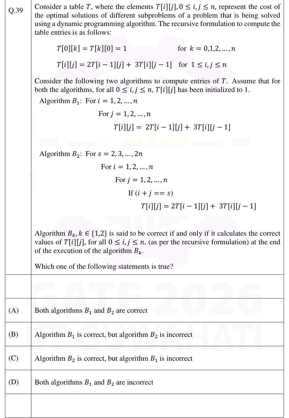
GATE 2026 CS2 Q.39

GATE 2026 · CS2Q.39 · 2 marks · MCQ

Consider a table $T$ , where the elements $T [i] [j]$ , $0 \leq i, j \leq n$ , represent the cost of the optimal solutions of different subproblems of a problem that is being solved using a dynamic programming algorithm. The recursive formulation to compute the table entries is as follows:

$T [0] [k] = T [k] [0] = 1 for k = 0, 1, 2, \dots, n$
$T [i] [j] = 2 T [i - 1] [j] + 3 T [i] [j - 1] for 1 \leq i, j \leq n$

Consider the following two algorithms to compute entries of $T$ . Assume that for both the algorithms, for all $0 \leq i, j \leq n$ , $T [i] [j]$ has been initialized to 1.

Algorithm $B_{1}$ :

For i = 1, 2, ..., n
    For j = 1, 2, ..., n
        T[i][j] = 2T[i-1][j] + 3T[i][j-1]

Algorithm $B_{2}$ :

For s = 2, 3, ..., 2n
    For i = 1, 2, ..., n
        For j = 1, 2, ..., n
            If (i + j == s)
                T[i][j] = 2T[i-1][j] + 3T[i][j-1]

Algorithm $B_{k}$ , $k \in {1, 2}$ is said to be correct if and only if it calculates the correct values of $T [i] [j]$ , for all $0 \leq i, j \leq n$ , (as per the recursive formulation) at the end of the execution of the algorithm $B_{k}$ .

Which one of the following statements is true?

(A)
Both algorithms $B_{1}$ and $B_{2}$ are correct
(B)
Algorithm $B_{1}$ is correct, but algorithm $B_{2}$ is incorrect
(C)
Algorithm $B_{2}$ is correct, but algorithm $B_{1}$ is incorrect
(D)
Both algorithms $B_{1}$ and $B_{2}$ are incorrect

Answer and solution

GATE 2026 CS2 Q.39: answer and solution

See the question in the paper

Tap to open full size

GATE 2026 CS2 Q.39: answer and solution

GATE 2026 DA Q.15

GATE 2026 · DAQ.15 · 1 mark · MCQ

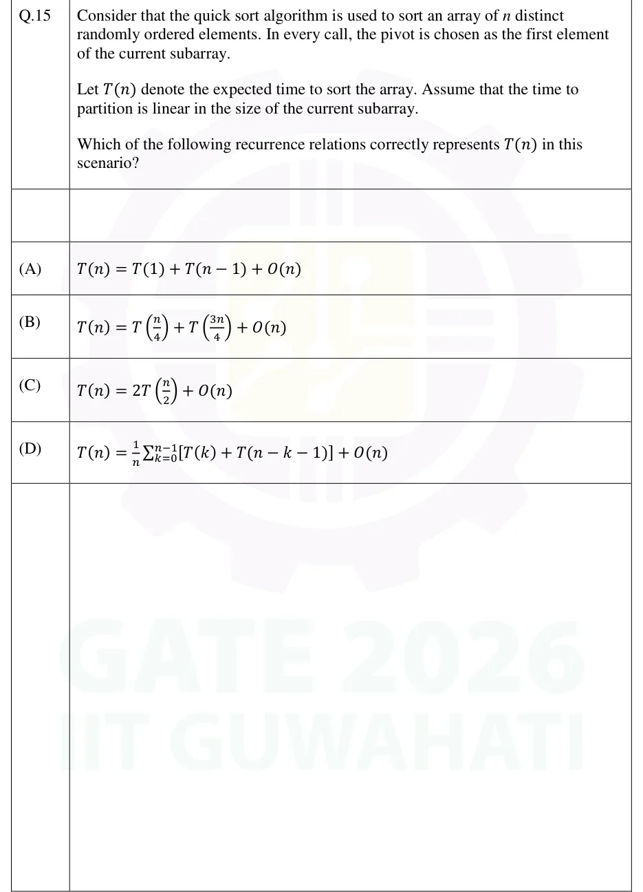
Consider that the quick sort algorithm is used to sort an array of $n$ distinct randomly ordered elements. In every call, the pivot is chosen as the first element of the current subarray.

Let $T (n)$ denote the expected time to sort the array. Assume that the time to partition is linear in the size of the current subarray.

Which of the following recurrence relations correctly represents $T (n)$ in this scenario?

(A)
$T (n) = T (1) + T (n - 1) + O (n)$
(B)
$T (n) = T (\frac{n}{4}) + T (\frac{3 n}{4}) + O (n)$
(C)
$T (n) = 2 T (\frac{n}{2}) + O (n)$
(D)
$T (n) = \frac{1}{n} \sum_{k = 0}^{n - 1} [T (k) + T (n - k - 1)] + O (n)$

Answer and solution

GATE 2026 DA Q.15: answer and solution

See the question in the paper

Tap to open full size

GATE 2026 DA Q.15: answer and solution

GATE 2024 CS2 Q.35

GATE 2024 · CS2Q.35 · 1 mark · NAT

Let $A$ be an array containing integer values. The distance of $A$ is defined as the minimum number of elements in $A$ that must be replaced with another integer so that the resulting array is sorted in non-decreasing order. The distance of the array $[2, 5, 3, 1, 4, 2, 6]$ is ____________.

Answer and solution

GATE 2024 CS2 Q.35: answer and solution

See the question in the paper

Tap to open full size

GATE 2024 CS2 Q.35: answer and solution

GATE 2024 CS2 Q.42

GATE 2024 · CS2Q.42 · 2 marks · MCQ

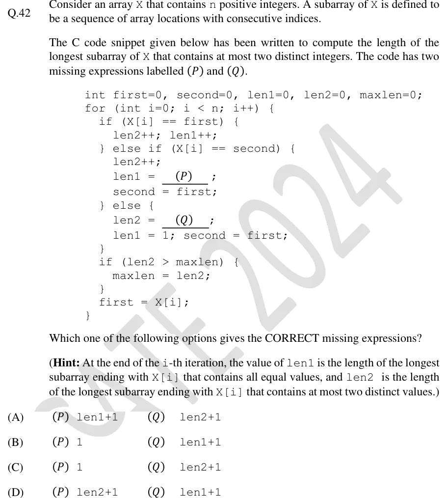
Consider an array X that contains n positive integers. A subarray of X is defined to be a sequence of array locations with consecutive indices.

The C code snippet given below has been written to compute the length of the longest subarray of X that contains at most two distinct integers. The code has two missing expressions labelled (P) and (Q).

int first=0, second=0, len1=0, len2=0, maxlen=0;
for (int i=0; i < n; i++) {
  if (X[i] == first) {
    len2++; len1++;
  } else if (X[i] == second) {
    len2++;
    len1 = (P) ;
    second = first;
  } else {
    len2 = (Q) ;
    len1 = 1; second = first;
  }
  if (len2 > maxlen) {
    maxlen = len2;
  }
  first = X[i];
}

Which one of the following options gives the CORRECT missing expressions?

(Hint: At the end of the i-th iteration, the value of len1 is the length of the longest subarray ending with X[i] that contains all equal values, and len2 is the length of the longest subarray ending with X[i] that contains at most two distinct values.)

(A)
(P) len1+1 (Q) len2+1
(B)
(P) 1 (Q) len1+1
(C)
(P) 1 (Q) len2+1
(D)
(P) len2+1 (Q) len1+1

Answer and solution

GATE 2024 CS2 Q.42: answer and solution

See the question in the paper

Tap to open full size

GATE 2024 CS2 Q.42: answer and solution

GATE 2024 DA Q.30

GATE 2024 · DAQ.30 · 1 mark · NAT

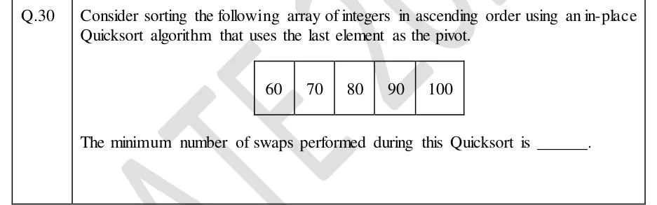
Consider sorting the following array of integers in ascending order using an in-place Quicksort algorithm that uses the last element as the pivot.

| 60 | 70 | 80 | 90 | 100 |

The minimum number of swaps performed during this Quicksort is ______.

Answer and solution

GATE 2024 DA Q.30: answer and solution

GATE 2023 CS Q.55

GATE 2023 · CSQ.55 · 2 marks · MSQ

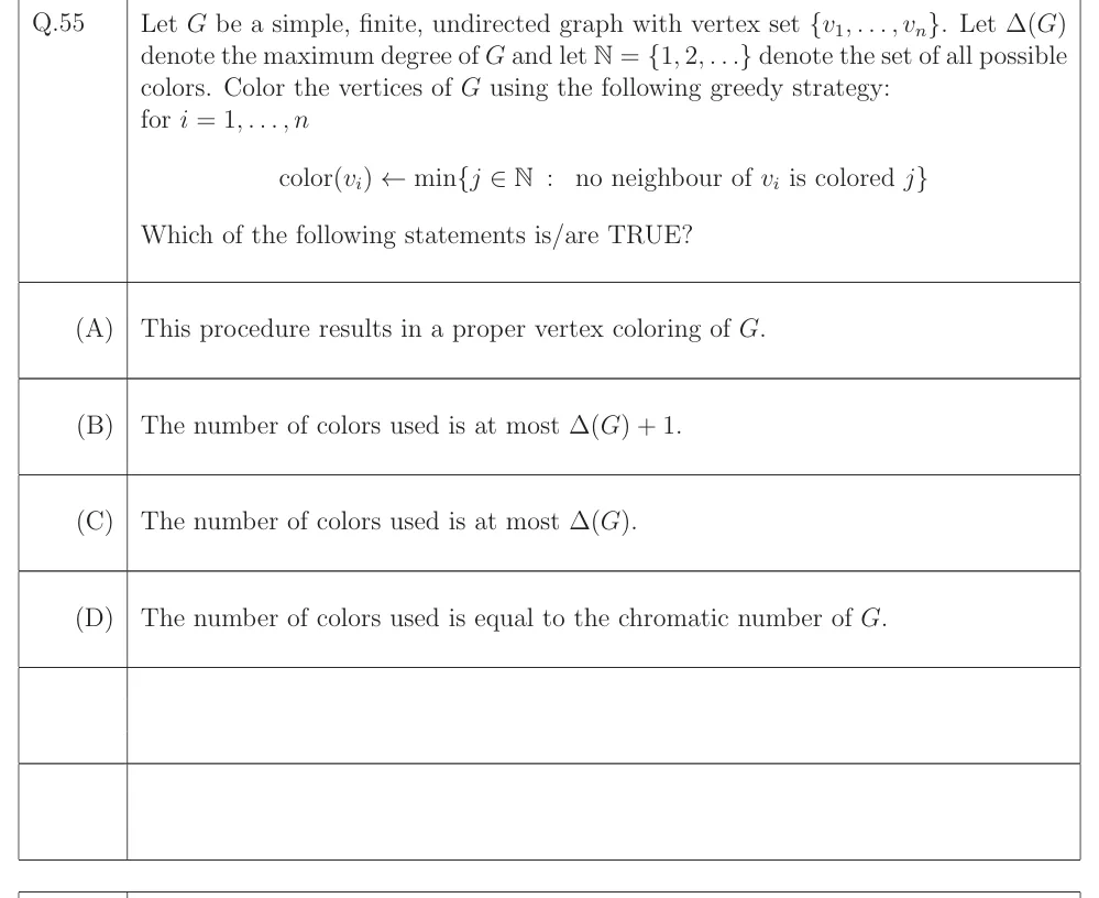
Let $G$ be a simple, finite, undirected graph with vertex set ${v_{1}, \dots, v_{n}}$ . Let $Δ (G)$ denote the maximum degree of $G$ and let $N = {1, 2, \dots}$ denote the set of all possible colors. Color the vertices of $G$ using the following greedy strategy:

for $i = 1, \dots, n$

color (v_{i}) \leftarrow min {j \in N : no neighbour of v_{i} is colored j}

Which of the following statements is/are TRUE?

(A)
This procedure results in a proper vertex coloring of $G$ .
(B)
The number of colors used is at most $Δ (G) + 1$ .
(C)
The number of colors used is at most $Δ (G)$ .
(D)
The number of colors used is equal to the chromatic number of $G$ .

Answer and solution

GATE 2023 CS Q.55: answer and solution

See the question in the paper

Tap to open full size

GATE 2023 CS Q.55: answer and solution

GATE 2018 CS Q.31

GATE 2018 · CSQ.31 · 2 marks · MCQ

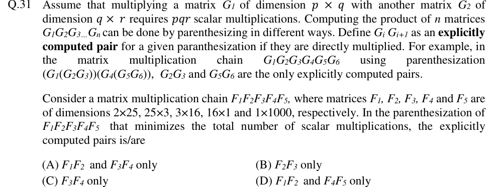
Assume that multiplying a matrix $G_{1}$ of dimension $p \times q$ with another matrix $G_{2}$ of dimension $q \times r$ requires $pq r$ scalar multiplications. Computing the product of $n$ matrices $G_{1} G_{2} G_{3} \dots G_{n}$ can be done by parenthesizing in different ways. Define $G_{i} G_{i + 1}$ as an explicitly computed pair for a given paranthesization if they are directly multiplied. For example, in the matrix multiplication chain $G_{1} G_{2} G_{3} G_{4} G_{5} G_{6}$ using parenthesization $(G_{1} (G_{2} G_{3})) (G_{4} (G_{5} G_{6}))$ , $G_{2} G_{3}$ and $G_{5} G_{6}$ are the only explicitly computed pairs.

Consider a matrix multiplication chain $F_{1} F_{2} F_{3} F_{4} F_{5}$ , where matrices $F_{1}, F_{2}, F_{3}, F_{4}$ and $F_{5}$ are of dimensions $2 \times 25$ , $25 \times 3$ , $3 \times 16$ , $16 \times 1$ and $1 \times 1000$ , respectively. In the parenthesization of $F_{1} F_{2} F_{3} F_{4} F_{5}$ that minimizes the total number of scalar multiplications, the explicitly computed pairs is/are

(A)
F1F2 and F3F4 only
(B)
F2F3 only
(C)
F3F4 only
(D)
F1F2 and F4F5 only

Answer and solution

GATE 2018 CS Q.31: answer and solution

See the question in the paper

Tap to open full size

GATE 2018 CS Q.31: answer and solution

GATE 2018 CS Q.48

GATE 2018 · CSQ.48 · 2 marks · NAT

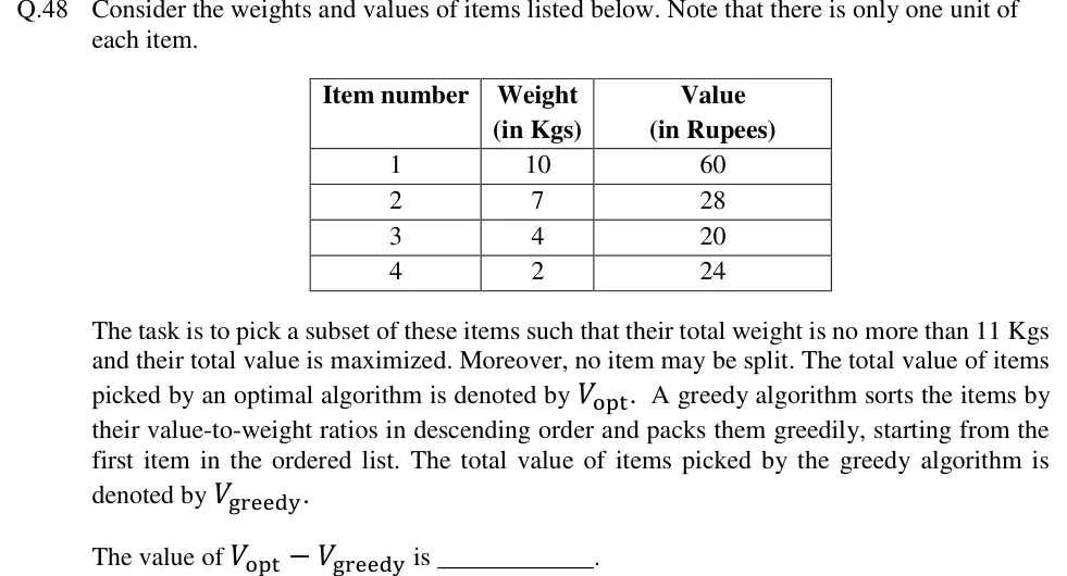
Consider the weights and values of items listed below. Note that there is only one unit of each item.

| Item number | Weight (in Kgs) | Value (in Rupees) |
|---|---|---|
| 1 | 10 | 60 |
| 2 | 7 | 28 |
| 3 | 4 | 20 |
| 4 | 2 | 24 |

The task is to pick a subset of these items such that their total weight is no more than 11 Kgs and their total value is maximized. Moreover, no item may be split. The total value of items picked by an optimal algorithm is denoted by $V_{o pt}$ . A greedy algorithm sorts the items by their value-to-weight ratios in descending order and packs them greedily, starting from the first item in the ordered list. The total value of items picked by the greedy algorithm is denoted by $V_{g r ee d y}$ .

The value of $V_{o pt} - V_{g r ee d y}$ is ____________.

Answer and solution

GATE 2018 CS Q.48: answer and solution

See the question in the paper

Tap to open full size

GATE 2018 CS Q.48: answer and solution

PRACTICE

6 questions to test yourself

PRACTICE 11 mark · MCQ

In the activity selection problem, the task is to select the maximum number of mutually compatible activities, each with a start and a finish time, on a single resource. The greedy strategy that is guaranteed to produce an optimal solution chooses the next activity by:

(A)
Earliest start time
(B)
Shortest duration
(C)
Earliest finish time
(D)
Maximum number of time overlaps with other activities

Answer and solution

Answer: (C)

Picking the compatible activity with the earliest finish time leaves the resource free from the earliest possible moment. Every activity that could follow any other choice can therefore also follow this one.
An exchange argument then shows that any optimal solution can have its first activity replaced by the earliest-finishing one without losing size.
Earliest start time and shortest duration lack this property. For example, one long activity starting first can block several short ones, and a short activity can overlap two others that are compatible with each other.
So the correct criterion is earliest finish time, which is why the standard algorithm begins by sorting on finish time.

PRACTICE 22 marks · NAT

A chain of 3 matrices A1, A2, A3 has dimensions A1: 10×20, A2: 20×5, A3: 5×15 (so p0=10, p1=20, p2=5, p3=15). Multiplying a p×q matrix by a q×r matrix costs pqr scalar multiplications. Using the matrix-chain-multiplication DP recurrence, what is the minimum number of scalar multiplications needed to compute A1·A2·A3?

Answer and solution

Answer: $1750$

Only two parenthesisations are possible for 3 matrices: (A1A2)A3 and A1(A2A3).
(A1A2)A3: cost(A1A2) = 10·20·5 = 1000, giving a 10×5 result; cost(result·A3) = 10·5·15 = 750. Total = 1000 + 750 = 1750.
A1(A2A3): cost(A2A3) = 20·5·15 = 1500, giving a 20×15 result; cost(A1·result) = 10·20·15 = 3000. Total = 1500 + 3000 = 4500.
In DP terms: m(1,2) = 1000 and m(2,3) = 1500, so m(1,3) = min(m(1,1) + m(2,3) + p0·p1·p3, m(1,2) + m(3,3) + p0·p2·p3) = min(0 + 1500 + 3000, 1000 + 0 + 750) = 1750.

PRACTICE 31 mark · MSQ

Which of the following problems are solved OPTIMALLY by a greedy algorithm, i.e. the greedy choice always leads to a globally optimal solution, with no need for dynamic programming?

(A)
Fractional Knapsack
(B)
0/1 Knapsack
(C)
Huffman Coding
(D)
Activity Selection

Answer and solution

Answer: (A), (C), (D)

Fractional knapsack: sorting by value/weight ratio and taking items greedily is provably optimal because items are divisible (an exchange argument on fractions works).
0/1 knapsack: greedy by ratio can be strictly worse than optimal because items are indivisible. Example: W=50 with items (10,60), (20,100), (30,120); greedy gets 160, the optimum is 220. It needs DP.
Huffman coding: repeatedly merging the two least frequent nodes is provably optimal (exchange argument on the two least frequent symbols).
Activity selection: the earliest-finish-time greedy is provably optimal (exchange argument, as in the first question).

PRACTICE 42 marks · NAT

Let X = "AGCAT" and Y = "GAC" (1-indexed; X has length 5 and Y has length 3). Using the standard LCS DP recurrence, what is the length of the Longest Common Subsequence of X and Y?

Answer and solution

Answer: $2$

Build the table L[i][j] for i = 0..5, j = 0..3 with L[i][0] = L[0][j] = 0.
Row i=1 (X1=A): L[1][1]=0 (A≠G), L[1][2]=1 (A=A), L[1][3]=1.
Row i=2 (X2=G): L[2][1]=1 (G=G), L[2][2]=1, L[2][3]=1.
Row i=3 (X3=C): L[3][1]=1, L[3][2]=1, L[3][3]=2 (C=C, L[2][2]+1).
Row i=4 (X4=A): L[4][1]=1, L[4][2]=2 (A=A, L[3][1]+1), L[4][3]=2.
Row i=5 (X5=T): L[5][1]=1, L[5][2]=2, L[5][3]=2 (no match, so the larger of the cell above and the cell to the left).
L[5][3] = 2, so the LCS length is 2 (e.g. "AC", "GC" or "GA"). "GAC" is not a subsequence of X, because no C comes after the A at position 4.

PRACTICE 51 mark · MCQ

Counting the number of inversions in an array of n distinct elements is done by a modified merge sort that counts, during each merge step, the pairs contributed across the two halves. The worst-case time complexity of this algorithm is:

(A)
O(n)
(B)
O(n log n)
(C)
O(n^2)
(D)
O(n^2 log n)

Answer and solution

Answer: (B)

The algorithm has the same recurrence as ordinary merge sort: T(n) = 2T(n/2) + Θ(n). The extra counting during a merge is O(1) per element placed, so each merge is still linear.
By case 2 of the master theorem (or O(n) work at each of O(log n) levels), T(n) = Θ(n log n).
Checking every pair also counts inversions, but takes Θ(n^2); the merge-based method is asymptotically faster.

PRACTICE 61 mark · MCQ

A divide-and-conquer algorithm satisfies the recurrence T(n) = 4T(n/2) + n^2 for n > 1, with T(1) = 1. Its running time is:

(A)
Θ(n^2)
(B)
Θ(n^2 log n)
(C)
Θ(n^3)
(D)
Θ(n log n)

Answer and solution

Answer: (B)

Here a = 4 and b = 2, so n^(log_b a) = n^(log_2 4) = n^2.
f(n) = n^2 = Θ(n^(log_b a)), which is case 2 of the master theorem.
So T(n) = Θ(n^2 log n). Check with a recursion tree: each level does 4^k · (n/2^k)^2 = n^2 work, and there are log_2 n + 1 levels.

OFFICIAL GATE 2027 SYLLABUS WORDING

Copied from the GATE 2027 syllabus; see all 2027 syllabi.

GATE CS

Algorithm design techniques: greedy, dynamic programming and divide‐and‐conquer

GATE DA

divide and conquer: mergesort, quicksort

Preparing in Kolkata? IAE Academy's course for GATE CSE or GATE DA.