GATE DA

Reasoning under uncertainty

Conditional independence, variable elimination and sampling

Reasoning under uncertainty represents a joint distribution compactly with a Bayesian network, uses conditional independence (read off by d-separation) to cut the number of parameters, and answers queries either exactly (enumeration, variable elimination) or approximately (prior, rejection, likelihood-weighting and Gibbs sampling). Typical problems ask you to factorise a joint, count parameters, decide whether two variables are independent given some evidence, run a small elimination or compute a sampling estimate by hand.

3 previous-year questions · 3 solved · 7 practice questions

Probability tools for reasoning

A joint distribution $P (X_{1}, \dots, X_{n})$ assigns a probability to every full assignment of the variables. Every other quantity is obtained from it by two operations: marginalisation (summing variables out) and conditioning (fixing observed variables and renormalising). Convention: $P (A ∣ B)$ is the probability of $A$ given $B$ , and $P (A, B)$ is the probability of both.

PRODUCT RULE

P (A, B) = P (A ∣ B) P (B) = P (B ∣ A) P (A)

Each conditional is defined only when the event it conditions on has positive probability ( $P (B) > 0$ for $P (A ∣ B)$ ).

MARGINALISATION (SUM RULE)

P (X) = y \sum P (X, y)

Sum over every value of each variable being removed.

BAYES' RULE

P (A ∣ B) = \frac{P ( B ∣ A ) P ( A )}{P ( B )}, P (B) = a \sum P (B ∣ a) P (a)

Requires $P (B) > 0$ . Turns a likelihood $P (B ∣ A)$ into a posterior $P (A ∣ B)$ ; the denominator comes from marginalisation.

CONDITIONING BY NORMALISATION

P (X ∣ e) = α P (X, e), α = \frac{1}{\sum _{x} P ( x , e )}

Requires $P (e) > 0$ . Compute the unnormalised values $P (x, e)$ for each $x$ , then divide by their sum. $α$ is just $1/ P (e)$ .

CHAIN RULE OF PROBABILITY

P (X_{1}, \dots, X_{n}) = i = 1 \prod n P (X_{i} ∣ X_{1}, \dots, X_{i - 1})

Holds for any distribution and any variable ordering (wherever the conditionals are defined); it is the starting point for the Bayesian-network factorisation.

EXAM TIP

A full joint over $n$ binary variables has $2^{n} - 1$ free numbers. That exponential size is the reason networks, conditional independence and clever inference exist.

Independence and conditional independence

$A$ and $B$ are independent if learning $B$ never changes belief about $A$ . They are conditionally independent given $C$ if, once $C$ is known, learning $B$ does not change belief about $A$ . Conditional independence is the structural property a Bayesian network encodes.

INDEPENDENCE

A ⊥ ⊥ B ⟺ P (A, B) = P (A) P (B) ⟺ P (A ∣ B) = P (A)

Must hold for every pair of values of $A$ and $B$ ; the last form is for values with $P (B) > 0$ .

CONDITIONAL INDEPENDENCE

A ⊥ ⊥ B ∣ C ⟺ P (A, B ∣ C) = P (A ∣ C) P (B ∣ C) ⟺ P (A ∣ B, C) = P (A ∣ C)

Must hold for every value of $A$ , $B$ and $C$ with $P (C) > 0$ (and $P (B, C) > 0$ for the last form).

Neither property implies the other. Two variables can be dependent marginally yet independent given a third (two effects of a common cause), and independent marginally yet dependent once a third is known (two independent causes of a common effect).

WORKED EXAMPLE

Binary $C$ with $P (C = 1) = 0.5$ . Given $C$ , $A$ and $B$ are independent with $P (A = 1 ∣ C = 1) = 0.8$ , $P (A = 1 ∣ C = 0) = 0.2$ , $P (B = 1 ∣ C = 1) = 0.8$ , $P (B = 1 ∣ C = 0) = 0.2$ . Are $A$ and $B$ independent when $C$ is not observed?

Solution

$P (A = 1, B = 1) = \sum_{c} P (c) P (A = 1 ∣ c) P (B = 1 ∣ c) = 0.5 (0.64) + 0.5 (0.04) = 0.34$ .
$P (A = 1) = 0.5 (0.8) + 0.5 (0.2) = 0.5$ , and likewise $P (B = 1) = 0.5$ , so $P (A = 1) P (B = 1) = 0.25$ .
$0.34 \neq = 0.25$ , so independence fails for this pair of values; $A$ and $B$ are dependent, although $A ⊥ ⊥ B ∣ C$ holds.

Answer: No. They are marginally dependent but conditionally independent given $C$ .

Bayesian networks and d-separation

A Bayesian network is a directed acyclic graph with one node per random variable and, for each node $X_{i}$ , a conditional probability table (CPT) $P (X_{i} ∣ Pa (X_{i}))$ giving its distribution for every assignment of its parents. A node with no parents has an ordinary (prior) table. The graph asserts that each variable is conditionally independent of its non-descendants given its parents (the local Markov property).

FACTORISATION OF THE JOINT IN A BAYESIAN NETWORK

P (X_{1}, \dots, X_{n}) = i = 1 \prod n P (X_{i} ∣ Pa (X_{i}))

For any choice of CPTs this product is a valid joint distribution, and a joint factorises this way exactly when it satisfies the local Markov property for the DAG. Any joint entry is the product of one CPT entry per node.

NUMBER OF INDEPENDENT CPT PARAMETERS

free parameters = i = 1 \sum n (∣ dom (X_{i}) ∣ - 1) X_{j} \in Pa (X_{i}) \prod ∣ dom (X_{j}) ∣

For all-binary variables this is $\sum_{i} 2^{∣ Pa (X_{i}) ∣}$ , compared with $2^{n} - 1$ for the full joint.

d-separation reads conditional independences from the graph. Look at every undirected path between $X$ and $Y$ , and examine each consecutive triple on it. Let $Z$ be the middle node and let the evidence set be the observed variables.

Triple	Shape	Blocked when	Open when
Chain	$X \to Z \to Y$ or $X \leftarrow Z \leftarrow Y$	$Z$ is observed	$Z$ is not observed
Fork (common cause)	$X \leftarrow Z \to Y$	$Z$ is observed	$Z$ is not observed
Collider (common effect)	$X \to Z \leftarrow Y$	$Z$ and all descendants of $Z$ are unobserved	$Z$ or any descendant of $Z$ is observed

Deciding whether X and Y are d-separated given evidence E

List every undirected path from $X$ to $Y$ (ignore arrow directions when walking; no node repeated on a path).
On each path, classify every consecutive triple as chain, fork or collider, and decide whether it is blocked given $E$ .
A path is blocked if at least one of its triples is blocked; a path is open only if all its triples are open.
$X$ and $Y$ are d-separated given $E$ if every path is blocked; then $X ⊥ ⊥ Y ∣ E$ holds in every distribution that factorises over the graph.
If some path is open, the graph does not guarantee independence (particular CPT values may still give it by accident).

MARKOV BLANKET

MB (X) = (Pa (X) \cup Children (X) \cup Pa (Children (X))) ∖ {X}

Parents, children and the children's other parents (co-parents). Given its Markov blanket, $X$ is conditionally independent of every other variable in the network.

WORKED EXAMPLE

Network $A \to B \to C$ with $P (A = 1) = 0.3$ , $P (B = 1 ∣ A = 1) = 0.8$ , $P (B = 1 ∣ A = 0) = 0.1$ , $P (C = 1 ∣ B = 1) = 0.9$ , $P (C = 1 ∣ B = 0) = 0.2$ . Find $P (A = 1, B = 0, C = 1)$ and the number of free parameters.

Solution

Factorise: $P (A, B, C) = P (A) P (B ∣ A) P (C ∣ B)$ .
$P (B = 0 ∣ A = 1) = 1 - 0.8 = 0.2$ and $P (C = 1 ∣ B = 0) = 0.2$ .
$P (A = 1, B = 0, C = 1) = 0.3 \times 0.2 \times 0.2 = 0.012$ .
Parameters: $A$ has 1, $B$ has 2, $C$ has 2, total 5 (the full joint needs 7).

Answer: $0.012$ ; the network has 5 free parameters.

EXAM TIP

A collider is the only triple that is blocked by default. Observing the collider, or any descendant of it, opens it: two independent causes become dependent once their common effect is known.

EXAM TIP

Edges need not be causal, and different DAGs can encode the same independences. $A \to B \to C$ , $A \leftarrow B \leftarrow C$ and $A \leftarrow B \to C$ all say exactly $A ⊥ ⊥ C ∣ B$ , whereas $A \to B \leftarrow C$ says $A ⊥ ⊥ C$ instead. In general two DAGs encode the same independences exactly when they have the same skeleton (edges ignoring direction) and the same v-structures (colliders $X \to Z \leftarrow Y$ with $X$ and $Y$ not adjacent).

Exact inference: enumeration and variable elimination

The inference task: given evidence $e$ on some variables, compute the posterior $P (Q ∣ e)$ of a query variable $Q$ . The remaining variables $H$ are hidden and must be summed out. Convention: ties in the elimination order are broken alphabetically unless a question gives an order; the final answer does not depend on the order, only the work does.

INFERENCE BY ENUMERATION

P (Q ∣ e) = α h \sum P (Q, e, h) = α h \sum i \prod P (X_{i} ∣ Pa (X_{i}))_{e}

Sum the network's joint over all hidden-variable assignments with evidence fixed, then normalise ( $P (e) > 0$ ). Cost is exponential in the number of hidden variables.

Variable elimination avoids repeating work by pushing each sum inwards. A factor is a table over a set of variables (a CPT is a factor). Two operations are used: the pointwise product of factors (multiply entries that agree on shared variables, result over the union of variables) and summing out a variable (add the entries over all its values, result over the remaining variables). Intermediate factors need not be probabilities.

ELIMINATING ONE VARIABLE

f^{'} (y) = x \sum k \prod f_{k} (x, y_{k})

Multiply only the factors that mention $X$ , then sum $X$ out; factors not mentioning $X$ are left untouched and can be pulled outside the sum.

Variable elimination procedure

Start with one factor per CPT.
Restrict every factor that mentions an evidence variable to its observed value (that variable disappears from the factor).
Choose an order for the hidden variables (alphabetical unless the question states one).
For each hidden variable $H$ in turn: multiply all current factors that contain $H$ , sum $H$ out, and put the new factor back in the pool.
When only factors over the query variable (and possibly constant factors with no variables) remain, multiply them and normalise to get $P (Q ∣ e)$ ; constant factors cancel in the normalisation.

Cost. The largest factor created decides the cost, and it depends on the elimination order. The cost is exponential in the number of variables in the largest factor created (the induced width of the order plus one). On a polytree (no undirected cycles, which includes chains and trees) a good order keeps factors small, so inference is linear in the size of the network (the total size of its CPTs); a bad order on the same network can be much worse. Computing the best order is hard in general, and exact inference in a general Bayesian network is NP-hard.

Pruning. A hidden variable that is not an ancestor of the query or of any evidence variable sums to 1 and can be deleted before starting; applying this repeatedly removes every such variable. Example: in $A \to B$ , $A \to C$ with query $A$ and evidence on $B$ , node $C$ is irrelevant.

WORKED EXAMPLE

Network $A \to B \to C$ with $P (A = 1) = 0.3$ , $P (B = 1 ∣ A = 1) = 0.8$ , $P (B = 1 ∣ A = 0) = 0.1$ , $P (C = 1 ∣ B = 1) = 0.9$ , $P (C = 1 ∣ B = 0) = 0.2$ . Use variable elimination (order $A$ , then $B$ ) to find $P (C = 1)$ .

Solution

Factors: $f_{1} (A) = P (A)$ , $f_{2} (A, B) = P (B ∣ A)$ , $f_{3} (B, C) = P (C ∣ B)$ .
Eliminate $A$ : $g (B) = \sum_{a} f_{1} (a) f_{2} (a, B)$ . $g (B = 1) = 0.3 (0.8) + 0.7 (0.1) = 0.24 + 0.07 = 0.31$ and $g (B = 0) = 0.3 (0.2) + 0.7 (0.9) = 0.06 + 0.63 = 0.69$ .
Eliminate $B$ : $h (C = 1) = \sum_{b} g (b) P (C = 1 ∣ b) = 0.31 (0.9) + 0.69 (0.2) = 0.279 + 0.138 = 0.417$ .
No evidence, so no normalisation is needed (and $h (C = 0) = 0.31 (0.1) + 0.69 (0.8) = 0.583$ confirms the total is 1).

Answer: $P (C = 1) = 0.417$

EXAM TIP

Do not forget to renormalise when there is evidence: the product of factors after restricting gives $P (Q, e)$ , not $P (Q ∣ e)$ . Divide by the sum over the values of $Q$ .

Approximate inference by sampling

When exact inference is too costly, estimate the posterior from random samples. Prior, rejection and likelihood-weighting sampling generate each variable in a topological order (parents before children) from its CPT given the already-sampled parents; Gibbs sampling instead resamples one variable at a time. The estimates are consistent (they converge to the true probability as the number of samples grows) but are only approximations for finite $N$ .

Convention for sampling by hand: for a binary variable, draw one random number $u$ uniform on $[0, 1)$ and set $X = 1$ if $u < P (X = 1 ∣ parents)$ , else $X = 0$ . Use the given random numbers in order, one per sampled variable, in topological order, unless the question states another rule.

PRIOR (FORWARD) SAMPLING

\hat{P} (x_{1}, \dots, x_{n}) = \frac{N ( x _{1} , \dots , x _{n} )}{N}

Each sample is drawn from the full joint, ignoring evidence; $N (\cdot)$ counts matching samples out of $N$ .

REJECTION SAMPLING

\hat{P} (Q = q ∣ e) = \frac{N ( q , e )}{N ( e )}

Generate prior samples, discard any that disagree with the evidence, and use the counts among the kept ones (undefined if $N (e) = 0$ ). The fraction kept is about $P (e)$ , so rare evidence wastes almost all samples.

WORKED EXAMPLE

Network $A \to B$ with $P (A = 1) = 0.4$ , $P (B = 1 ∣ A = 1) = 0.9$ , $P (B = 1 ∣ A = 0) = 0.2$ . Evidence $B = 1$ . Using the convention above, four samples use the random-number pairs $(u_{A}, u_{B})$ : $(0.25, 0.95)$ , $(0.70, 0.10)$ , $(0.35, 0.50)$ , $(0.85, 0.15)$ . Estimate $P (A = 1 ∣ B = 1)$ by rejection sampling.

Solution

Sample 1: $0.25 < 0.4$ so $A = 1$ ; $0.95 \geq 0.9$ so $B = 0$ . Rejected.
Sample 2: $0.70 \geq 0.4$ so $A = 0$ ; $0.10 < 0.2$ so $B = 1$ . Kept, $A = 0$ .
Sample 3: $0.35 < 0.4$ so $A = 1$ ; $0.50 < 0.9$ so $B = 1$ . Kept, $A = 1$ .
Sample 4: $0.85 \geq 0.4$ so $A = 0$ ; $0.15 < 0.2$ so $B = 1$ . Kept, $A = 0$ .
Kept 3 samples, one with $A = 1$ : estimate $1/3$ .

Answer: $\hat{P} (A = 1 ∣ B = 1) = 1/3 \approx 0.333$ (the exact value is $0.75$ ; four samples is very few).

LIKELIHOOD WEIGHTING

w = j \prod P (e_{j} ∣ Pa (E_{j})), \hat{P} (Q = q ∣ e) = \frac{\sum _{s : Q^{(s)} = q} w ^{(s)}}{\sum _{s} w ^{(s)}}

Evidence variables are fixed, not sampled; each sample is weighted by the probability of the evidence given its parents' values in that same sample (a parent may itself be an evidence variable, fixed at its observed value). Non-evidence variables are sampled as usual, so no sample is rejected. The method is consistent because the probability of drawing the non-evidence values $z$ times the weight equals $P (z, e)$ .

WORKED EXAMPLE

Network $A \to B$ with $P (A = 1) = 0.4$ , $P (B = 1 ∣ A = 1) = 0.9$ , $P (B = 1 ∣ A = 0) = 0.2$ . Evidence $B = 1$ . Five likelihood-weighting samples draw $A = 1, 0, 1, 1, 0$ from its prior. Estimate $P (A = 1 ∣ B = 1)$ and compare with the exact value.

Solution

Weight of a sample is $P (B = 1 ∣ A)$ : $0.9, 0.2, 0.9, 0.9, 0.2$ .
Weight with $A = 1$ : $0.9 + 0.9 + 0.9 = 2.7$ . Total weight: $2.7 + 0.2 + 0.2 = 3.1$ .
Estimate $= 2.7/3.1 \approx 0.871$ .
Exact: $P (A = 1, B = 1) = 0.36$ , $P (A = 0, B = 1) = 0.12$ , so $P (A = 1 ∣ B = 1) = 0.36/0.48 = 0.75$ . The estimate is off because five samples is small.

Answer: $\hat{P} \approx 0.871$ against the exact $0.75$ .

GIBBS SAMPLING: RESAMPLING ONE VARIABLE

P (x_{i} ∣ mb (X_{i})) = α P (x_{i} ∣ pa (X_{i})) Y_{j} \in Children (X_{i}) \prod P (y_{j} ∣ pa (Y_{j}))

All other variables are held at their current values; $α$ normalises over the values $x_{i}$ . Only the CPTs of $X_{i}$ and of its children are needed, because $X_{i}$ is independent of everything else given its Markov blanket.

Gibbs sampling procedure (an MCMC method)

Fix the evidence variables at their observed values and give every non-evidence variable an initial value.
Repeatedly pick a non-evidence variable $X_{i}$ (in a fixed order or at random) and resample it from $P (X_{i} ∣ mb (X_{i}))$ using the current values of the others.
Each resulting full state is one sample; estimate $P (Q = q ∣ e)$ as the fraction of states with $Q = q$ .

WORKED EXAMPLE

Network $A \to B \to C$ with $P (A = 1) = 0.3$ , $P (B = 1 ∣ A = 1) = 0.8$ , $P (B = 1 ∣ A = 0) = 0.1$ , $P (C = 1 ∣ B = 1) = 0.9$ , $P (C = 1 ∣ B = 0) = 0.2$ . Evidence $C = 1$ ; the current state has $A = 1$ . Gibbs sampling now resamples $B$ . With what probability is $B = 1$ drawn?

Solution

$MB (B) = {A, C}$ , so $P (b ∣ A = 1, C = 1) = α P (b ∣ A = 1) P (C = 1 ∣ b)$ .
$B = 1$ : $0.8 \times 0.9 = 0.72$ . $B = 0$ : $0.2 \times 0.2 = 0.04$ .
Normalise: $0.72/ (0.72 + 0.04) = 0.72/0.76 \approx 0.947$ .

Answer: $P (B = 1 ∣ A = 1, C = 1) \approx 0.947$

Method	Evidence handled by	Waste	Weakness
Prior sampling	Not used (estimates any event)	None, but evidence is not conditioned on	Cannot give a conditional probability by itself
Rejection sampling	Discarding inconsistent samples	Fraction $1 - P (e)$ of samples thrown away, on average	Very inefficient when $P (e)$ is small
Likelihood weighting	Fixing evidence and weighting	No samples discarded	Evidence influences only the sampling of variables downstream of it; upstream variables are drawn from their priors, so weights can become tiny when evidence is unlikely
Gibbs sampling	Fixing evidence; resampling each variable given its Markov blanket	No samples discarded	Successive samples are correlated; early samples depend on the starting state

EXAM TIP

In likelihood weighting the evidence variable is never sampled and the weight uses the CPT entry of the evidence given the sampled parents. In rejection sampling you do sample it and then throw the sample away if it differs from the evidence. Mixing these up changes the answer.

EXAM TIP

Gibbs estimates converge to the true posterior when the chain can reach every state; a sufficient condition is that every CPT entry is strictly positive. Early samples are often discarded (burn-in) because they still reflect the arbitrary starting state.

PREVIOUS-YEAR QUESTIONS

3 questions from the DA papers

Try each question first, then open the answer. We placed each question under a topic ourselves; the exam paper does not label topics.

See these papers in full: GATE DA 2025 · GATE DA 2024

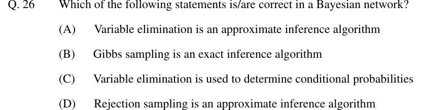
GATE 2025 DA Q.26

GATE 2025 · DAQ.26 · 1 mark · MSQ

Which of the following statements is/are correct in a Bayesian network?

(A)
Variable elimination is an approximate inference algorithm
(B)
Gibbs sampling is an exact inference algorithm
(C)
Variable elimination is used to determine conditional probabilities
(D)
Rejection sampling is an approximate inference algorithm

Answer and solution

GATE 2025 DA Q.26: answer and solution

See the question in the paper

Tap to open full size

GATE 2025 DA Q.26: answer and solution

GATE 2024 DA Q.24

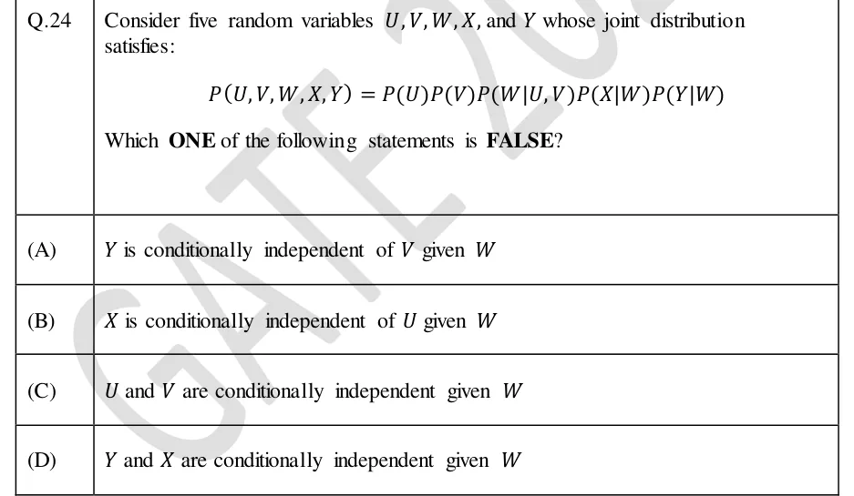
GATE 2024 · DAQ.24 · 1 mark · MCQ

Consider five random variables $U, V, W, X$ , and $Y$ whose joint distribution satisfies:

P (U, V, W, X, Y) = P (U) P (V) P (W ∣ U, V) P (X ∣ W) P (Y ∣ W)

Which ONE of the following statements is FALSE?

(A)
$Y$ is conditionally independent of $V$ given $W$
(B)
$X$ is conditionally independent of $U$ given $W$
(C)
$U$ and $V$ are conditionally independent given $W$
(D)
$Y$ and $X$ are conditionally independent given $W$

Answer and solution

GATE 2024 DA Q.24: answer and solution

See the question in the paper

Tap to open full size

GATE 2024 DA Q.24: answer and solution

GATE 2024 DA Q.64

GATE 2024 · DAQ.64 · 2 marks · NAT

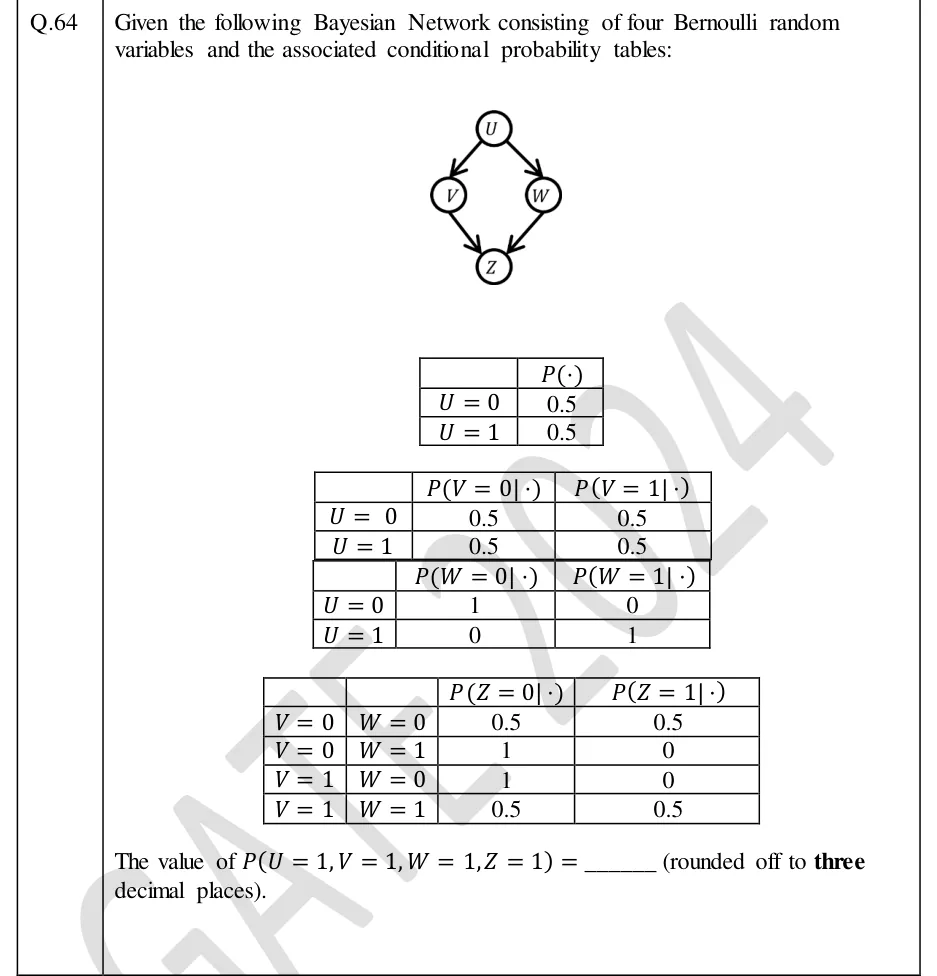
Given the following Bayesian Network consisting of four Bernoulli random variables and the associated conditional probability tables:

The value of $P (U = 1, V = 1, W = 1, Z = 1) =____$ (rounded off to three decimal places).

GATE 2024 DA question 64: Directed acyclic graph with four nodes U, V, W, Z. — Figure from the GATE 2024 DA paper. It is part of the question.

Answer and solution

GATE 2024 DA Q.64: answer and solution

PRACTICE

7 questions to test yourself

PRACTICE 11 mark · MCQ

In the Bayesian network with edges $A \to C$ , $B \to C$ and $C \to D$ , which statement is guaranteed by the graph?

(A)
$A ⊥ ⊥ B ∣ C$
(B)
$A ⊥ ⊥ B ∣ D$
(C)
$A ⊥ ⊥ B$ (nothing observed)
(D)
$A ⊥ ⊥ D$ (nothing observed)

Answer and solution

Answer: (C)

The only path between $A$ and $B$ is $A \to C \leftarrow B$ , a collider at $C$ .
With nothing observed the collider is blocked, so $A ⊥ ⊥ B$ holds: option C.
Observing $C$ opens the collider, so A is false; observing $D$ , a descendant of $C$ , also opens it, so B is false.
$A \to C \to D$ is an open chain when nothing is observed, so $A$ and $D$ are not guaranteed independent: D is false.

PRACTICE 21 mark · NAT

Five binary variables $A, B, C, D, E$ form a Bayesian network with edges $A \to C$ , $B \to C$ , $C \to D$ and $C \to E$ . How many independent parameters are needed to specify all the CPTs?

Answer and solution

Answer: $10$

Each binary node needs $2^{∣ Pa ∣}$ parameters.
$A$ : 1, $B$ : 1, $C$ (two binary parents): 4, $D$ (one parent): 2, $E$ (one parent): 2.
Total $1 + 1 + 4 + 2 + 2 = 10$ (the full joint would need $2^{5} - 1 = 31$ ).

PRACTICE 32 marks · NAT

Network $A \to B \to C$ of binary variables with $P (A = 1) = 0.5$ , $P (B = 1 ∣ A = 1) = 0.6$ , $P (B = 1 ∣ A = 0) = 0.2$ , $P (C = 1 ∣ B = 1) = 0.7$ , $P (C = 1 ∣ B = 0) = 0.1$ . Using variable elimination, compute $P (A = 1 ∣ C = 1)$ . Give the answer correct to 3 decimal places.

Answer and solution

Answer: $0.676$ (accepted range $\pm 0.001$ )

Restrict to $C = 1$ : $f (B) = P (C = 1 ∣ B)$ gives $f (1) = 0.7$ , $f (0) = 0.1$ .
Eliminate $B$ for each value of $A$ : $g (A = 1) = 0.6 (0.7) + 0.4 (0.1) = 0.46$ and $g (A = 0) = 0.2 (0.7) + 0.8 (0.1) = 0.22$ .
Multiply by the prior: $P (A = 1, C = 1) = 0.5 (0.46) = 0.23$ and $P (A = 0, C = 1) = 0.5 (0.22) = 0.11$ .
Normalise: $P (A = 1 ∣ C = 1) = 0.23/ (0.23 + 0.11) = 0.23/0.34 \approx 0.676$ .

PRACTICE 41 mark · NAT

Network $A \to B$ with $P (A = 1) = 0.4$ , $P (B = 1 ∣ A = 1) = 0.9$ , $P (B = 1 ∣ A = 0) = 0.2$ . Rejection sampling with evidence $B = 1$ is run on 2000 independent prior samples. What is the expected number of samples that are kept?

Answer and solution

Answer: $960$

A sample is kept exactly when its $B$ value equals the evidence, which has probability $P (B = 1)$ .
$P (B = 1) = 0.4 (0.9) + 0.6 (0.2) = 0.36 + 0.12 = 0.48$ .
Expected kept samples $= 2000 \times 0.48 = 960$ .

PRACTICE 51 mark · MCQ

A Bayesian network has edges $A \to C$ , $B \to C$ , $C \to D$ , $E \to D$ and $D \to F$ . What is the Markov blanket of $C$ ?

(A)
${A, B, D}$
(B)
${A, B, D, E}$
(C)
${A, B, D, E, F}$
(D)
${D, E, F}$

Answer and solution

Answer: (B)

Parents of $C$ : ${A, B}$ .
Children of $C$ : ${D}$ .
Other parents of the child $D$ : ${E}$ ( $C$ itself is excluded).
$MB (C) = {A, B, D, E}$ . $F$ is a grandchild and is not in the blanket: option B.

PRACTICE 62 marks · NAT

Binary network with edges $A \to B$ and $C \to B$ : $P (A = 1) = 0.2$ , $P (C = 1) = 0.6$ , $P (B = 1 ∣ A = 1, C = 1) = 0.9$ , $P (B = 1 ∣ A = 1, C = 0) = 0.7$ , $P (B = 1 ∣ A = 0, C = 1) = 0.4$ , $P (B = 1 ∣ A = 0, C = 0) = 0.1$ . Evidence $B = 1$ . In Gibbs sampling the current state has $C = 0$ , and $A$ is now resampled. With what probability is $A = 1$ drawn? Give the answer correct to 3 decimal places.

Answer and solution

Answer: $0.636$ (accepted range $\pm 0.001$ )

$MB (A) = {B, C}$ (child $B$ and co-parent $C$ ), so $P (a ∣ B = 1, C = 0) = α P (a) P (B = 1 ∣ a, C = 0)$ .
$A = 1$ : $0.2 \times 0.7 = 0.14$ . $A = 0$ : $0.8 \times 0.1 = 0.08$ .
Normalise: $0.14/ (0.14 + 0.08) = 0.14/0.22 \approx 0.636$ .

PRACTICE 72 marks · MSQ

Network with edges $A \to B$ , $B \to C$ , $A \to D$ and $D \to C$ . Select all statements that hold in every distribution that factorises over this graph.

(A)
$B ⊥ ⊥ D ∣ A$
(B)
$B ⊥ ⊥ D$ (nothing observed)
(C)
$B ⊥ ⊥ D ∣ {A, C}$
(D)
$A ⊥ ⊥ C ∣ {B, D}$

Answer and solution

Answer: (A), (D)

Option A: path $B \leftarrow A \to D$ is a fork blocked by observed $A$ ; path $B \to C \leftarrow D$ is a collider at unobserved $C$ (no observed descendants), blocked. True.
Option B: $B \leftarrow A \to D$ is an open fork when $A$ is unobserved. Not guaranteed.
Option C: observing $C$ opens the collider $B \to C \leftarrow D$ , so $B$ and $D$ can be dependent. Not guaranteed.
Option D: $A \to B \to C$ is blocked by observed $B$ , and $A \to D \to C$ is blocked by observed $D$ . True.

OFFICIAL GATE 2027 SYLLABUS WORDING

Copied from the GATE 2027 syllabus; see all 2027 syllabi.

GATE DA

reasoning under uncertainty topics — conditional independence representation, exact inference through variable elimination, and approximate inference through sampling

Preparing in Kolkata? IAE Academy's course for GATE DA.